
In a previous post I provided an overview of the Layout of an Excel Workbook and briefly discussed the Excel Ribbon, the part of the Workbook where many common Functions and Operations are found.
This post delves more into that topic and will give you a comprehensive guide to the Excel Ribbon, focusing on the Home Tab.
The Home Tab
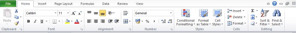
As we embark on a journey through Excel’s Ribbon, let’s start with the Home tab, a fundamental part of Excel.
When you open a new Excel workbook, the first thing you usually see is the Home tab. It’s not just the first in line; it’s the go-to place for many essential Excel commands you’ll use daily.
In this guide, we’re diving into the Excel Ribbon, focusing on the standard layout of the Home tab as you would see in a new Excel installation. This way, we can create a common ground for everyone, especially beginners.
So, whether you’re new to Excel or brushing up on the basics, our exploration starts here at the Home tab – your gateway to mastering Excel’s diverse features.
Tip: Hover the mouse cursor over any Icon on the Ribbon and a pop-up box will display what that Icon is for.
Command Groups
The various commands on the Home Tab are grouped in order to make the Ribbon as user-friendly as possible, the groupings listed are as follows (from left to right on the Ribbon):
- Clipboard
- Font
- Alignment
- Number
- Styles
- Cells
- Editing
Excel Download File
It is not required but if you don’t want the hassle of creating your own data or examples and would like to follow along with some of the tips then a sample workbook has been created, you can download this here.
The Clipboard Command Group
First up in our guide to the Excel Ribbon is the Clipboard Command Group. In this Command Group you have Icons for Cut, Copy, Paste and Format Painter and they come in very useful when working with data in an Excel Workbook:
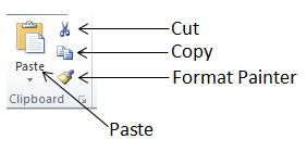
- Cut: This command cuts data in preparation to move it to another location in the Excel Workbook.
- Copy: This command copies data in preparation to copy it to another location in your Excel Workbook.
- Paste: When you have either Cut or Copied data then you use the Paste command to paste it to the new location.
- Format Painter: Not as intuitive as the others but this command will copy the format of a cell and allow you to quickly apply it to other cells in your Workbook. For example if you have a cell that is a certain font type and you want to apply that font type to other cells you would click on the cell to copy (making it active) and the click the Format Painter command. You then click on the cell(s) that you want to apply that format on and Excel takes care of the rest.
Tip: To highlight a range of cells click on the starting cell then hold the left mouse button down and drag the mouse to cover the range of cells you want to highlight. Excel will highlight the cells to show you what has been selected and any commands you then choose will apply to all the highlighted cells.
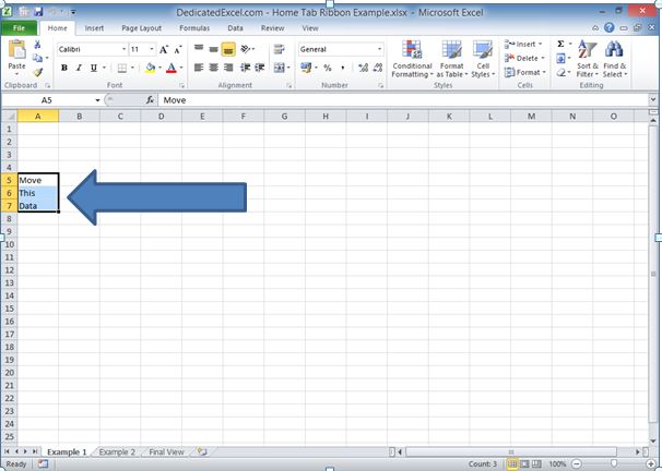
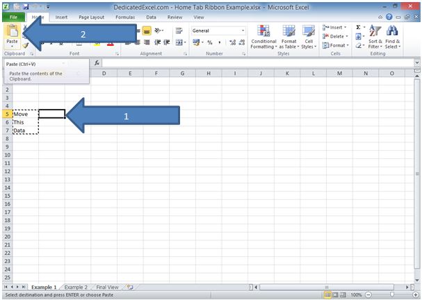
In the Example workbook you can see on Worksheet “Example 1” there is data in A5, A6 and A7 this can be moved by first clicking on Cell A5 then with the left mouse button pressed drag the cursor down to cell A7:
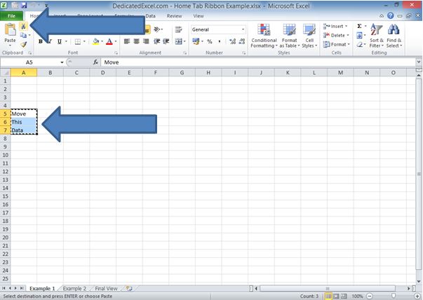
To move the data select the Cut command from the Excel Ribbon and Excel![]() while the cells remain highlighted. The selected cells will then have a moving dotted line around them, this indicates you are about to move these cells:
while the cells remain highlighted. The selected cells will then have a moving dotted line around them, this indicates you are about to move these cells:
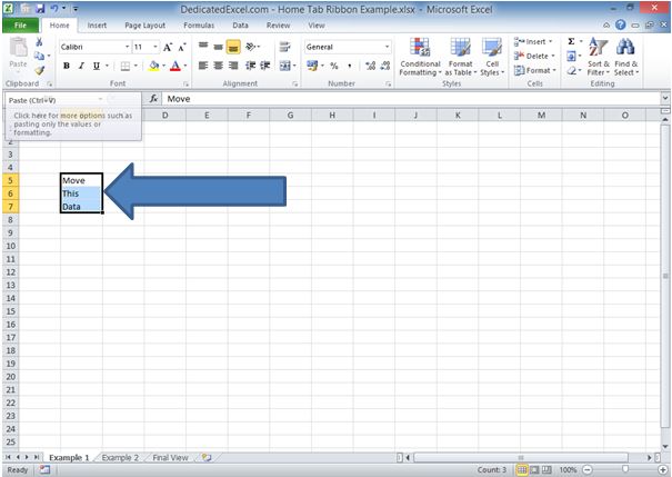
To move the data click on cell B5, making it the active cell, then click on Paste from the Excel Ribbon:
When you click Paste the data will have moved to the new location:
The Font Command Group
If you want to change the appearance of your cells then the Font Command Group is where you can perform those tasks.
Within the Font Command Group there are options to change the Font Type, Size and colour along with placing Borders around cells or even fill them some colour.
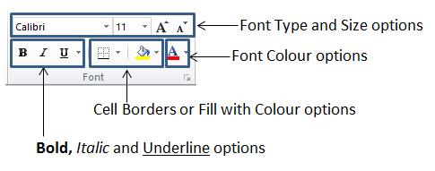
Take note of the small arrowheads next to some of the Command icons as this indicates there are various sub-options that are available.
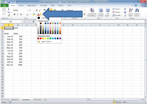
For example when changing the Font Colour you can click on the arrowhead next to the Font Colour icon and this will bring up the Colour Palette allowing you to select your colour of choice:
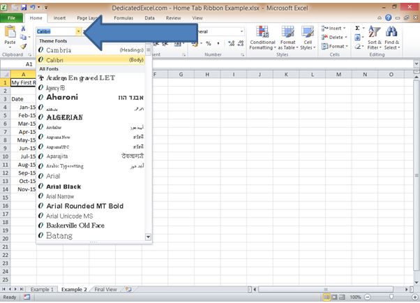
Alternatively if you need to change the Font Type click on the arrowhead next to the Font Type icon and this will show you the Fonts that are available:
Tip: Unless your company has a standard practice with regards to Fonts and Colour schemes then try to develop a style of your own and stick with it. If you are creating Worksheets for others, i.e. Reports, a well styled Worksheet with some colour can make your hard work stand out…just try not to go too overboard with the colours.
The Alignment Command Group
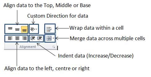
The Alignment Command Group is about changing the Alignment of data within a cell or range of cells. This means data can be aligned to appear at the top, middle or base of a cell along with aligning the data to the left, centre or right of a cell.
There are also options to make the data appear in a custom direction, for example diagonally, or merged across multiple cells on the Worksheet.
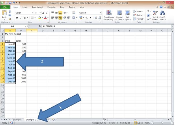
If you are following along with the downloaded examples file select the Worksheet “Example 2”. You will see the data table that the dates in Column A are all to the right of the cells, this is known as Right Alignment:
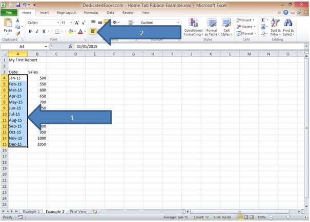
If you highlight all the date cells you can change the alignment to be from the left by clicking on the Align Left Icon in the Alignment Command Group.
The Number Command Group
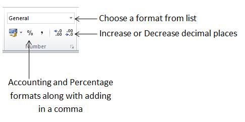
Next up on our guide to the Excel Ribbon is the Number Command Group. The Number Command Group is used for formatting numerical data.
There are options to change the number type to Accounting formats, Currencies or Percentages along with adding comma’s (thousand separators) and decimal places to better display your numerical data.
You can also format the data for dates or even create your own custom number format:
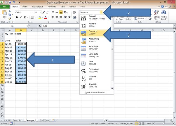
Using the downloaded example file on worksheet “Example 2” convert the Sales data into Currency format by highlighting the cells and selecting the Currency data type from the drop down menu.
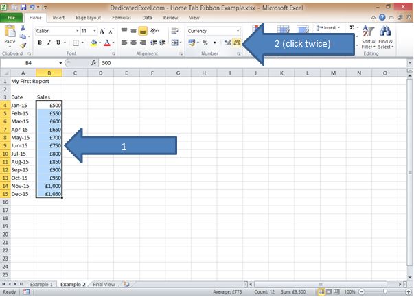
Next remove the decimal places by keeping the cells highlighted and clicking on the Decrease Decimal Icon.
In this case the Currency has two decimal places (two numbers after the decimal) so click on the Decrease Decimal button twice to remove it completely.
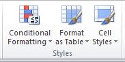
The Styles Command Group
If there are no standard practices for Worksheet style or you don’t wish to develop your own then Excel provides custom styles that you can use on your data, the Styles Command group contains some of these features.
Conditional Formatting is also included in this group and that is a command where you can set format styles based on rules you create.
For example if a cell value is greater than zero you could make the cell green, this type of technique comes in handy for Traffic Light Reports and creating Excel Dashboards.
The Format as Table command takes a range of data and applies a Table format to it. In the downloaded example file on worksheet “Example 2” click on the Format as Table icon.
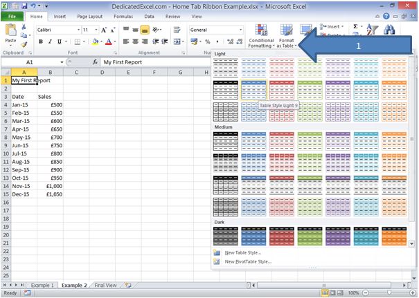
An array of table styles will appear all with unique colour and formatting schemes, select the one you want to apply.
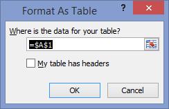
The ‘Format As Table’ box will then pop-up asking you where the data is for your table and whether your table has headers:
The data for the example is contained in cells A3 to B15 and it has headers so you would input those details like below:
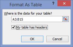
Note the Colon punctuation mark is used in Excel to specify a range so A3 to B15 is written as A3:B15
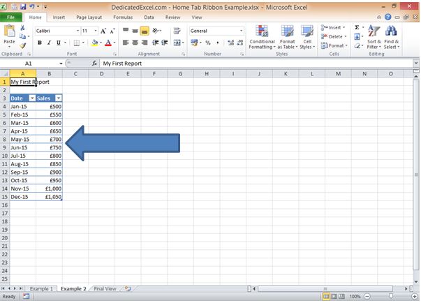
Click OK and the Table style selected will be applied to the data:
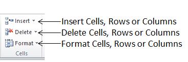
The Cells Command Group
The Cells Command Group is used when you need to insert or remove cells, rows or columns in the worksheet.
There are also options to Format Cells to auto-fit a column which can make your reports appear more professional and easier on the eye.
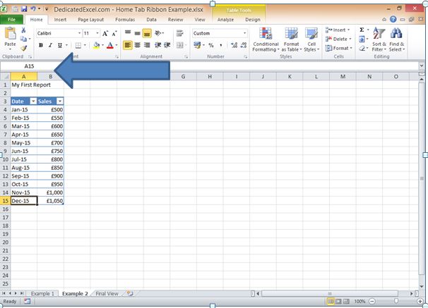
In the downloaded example file on the “Example 2” Worksheet notice how the title in cell A1 goes across to column B as it is too long for the column width:
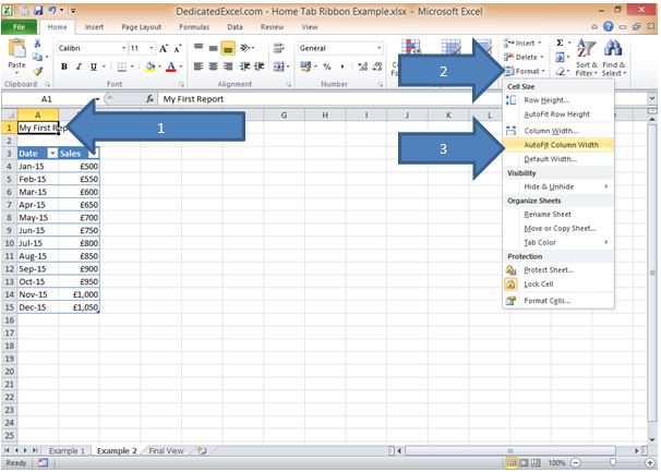
Format the width of Column A so the title “My First Report” does not go across column B. Start by clicking on cell A1 to make that the active cell, then select Format and “AutoFit Column Width” from the options box:
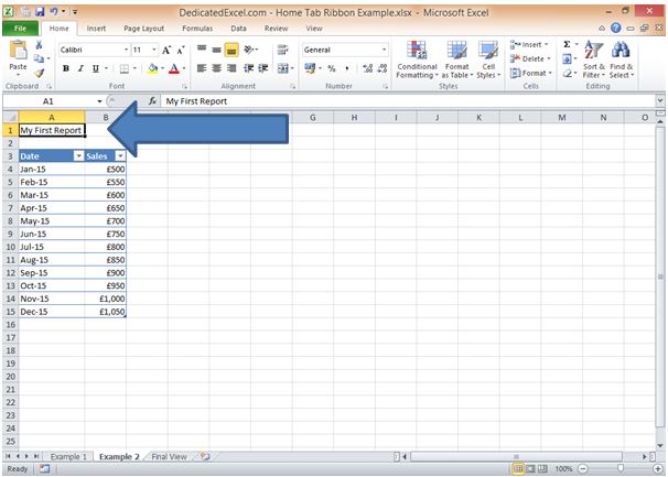
After you have clicked on “AutoFit Column Width” notice Column A has adjusted and the Title no longer goes across Column B:
Next remove Row 15 from the Table, which contains Dec-15 data, by first clicking on cell A15 and selecting “Delete Table Rows” from the Delete Command:
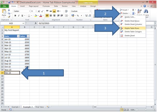
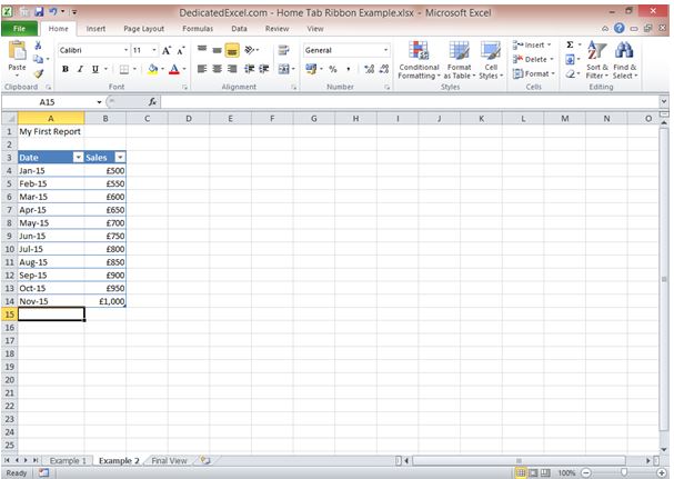
When you have clicked “Delete Table Rows” notice that the data in Row 15 has now been deleted:
Note: Row 15 on the Worksheet is not deleted from existence (you can’t do that) but the data and any formatting in Row 15 is removed.
The Editing Command Group
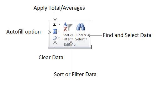
Last on the list of our guide to the Excel Ribbon – Home tab is the Editing Command Group. This has some useful features that will help you when you have tables of data or Worksheets with lots of information to review and work with.
There are commands to insert totals or averages, AutoFill data (which can be used for creating datasets) and to clear data from Worksheet cells.
You can also sort or apply filters to your data tables and use the “Find & Select” command to search quickly for information in a Worksheet.
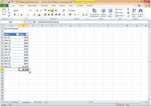
On the “Example 2” Worksheet add a Total to the Sales Column by Clicking on Cell B15 then Clicking on the SUM Command and selecting SUM from the options box:
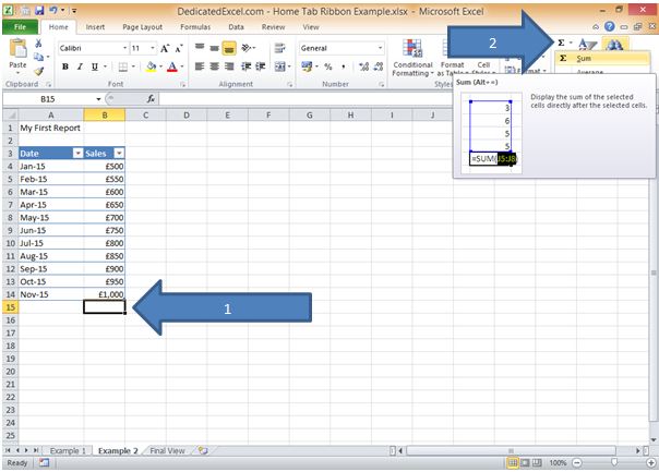
A Total is applied to that column. Note that Excel will do its best to make life simple and it will automatically assume you want to total Column B as you have made cell B15 your active cell.
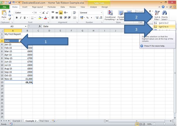
Next you can sort the data so the most recent month appears first by clicking on cell A3 (Date), then clicking on the Sort & Filter command and selecting “Sort Z to A” from the options box:
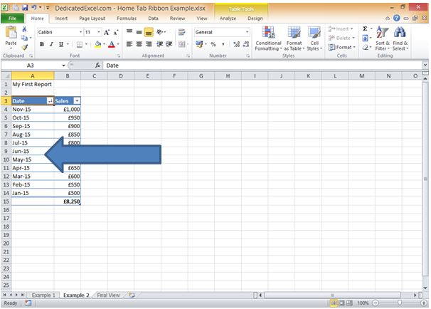
The data will now show with the most recent date first, to revert it back to oldest date first you would choose the Sort A to Z option:
On the downloadable examples file you click on the Worksheet “Final View” to see how your Worksheet should now look.
Don’t worry if you haven’t got everything exact, the important thing is that you have learned a lot of new information by reading and working through this post, you can always review again when you have time.
Summary
Thank you for joining me through this detailed exploration in our guide to the Excel Ribbon, focusing on the multifaceted Home Tab. We’ve covered everything from the basics of clipboard and font commands to the more intricate aspects of cell formatting and data editing.
This guide provides you with a thorough understanding of the most commonly used tab on the Excel ribbon. By working through the examples provided, you’ve taken significant strides in advancing your Excel proficiency, moving beyond the novice level.
Our journey through the Home Tab exemplifies just how versatile and powerful Excel can be when you fully utilize its tools. As you continue to apply these insights and techniques, you’ll find yourself navigating Excel with greater ease and confidence.
The knowledge gained here lays a strong foundation for further exploring the extensive capabilities of Excel, ensuring you’re well-equipped for any task at hand.
Keep Excelling,

If this guide to the Excel ribbon has left you thirsty for more Excel knowledge how about something a little quicker, but just as useful, with our guide on how to create your own Excel function.