
Navigating through extensive datasets in Excel can be daunting, but the freeze panes in Excel feature is a game-changer. This technique allows you to lock specific rows or columns in place, ensuring key information remains visible as you scroll through your data. This guide will detail how to effectively freeze panes in Excel to enhance your data viewing and interaction experience.
Introduction
Excel’s capability to manage large datasets, like a table with 50 columns or a log of 10 years of daily share prices, is unparalleled. But presenting such vast amounts of data in a single worksheet can often challenge user-friendliness.
This is where the skill to freeze panes in Excel becomes not just useful, but essential, allowing for a more manageable and efficient data review process.
Freezing Panes in Excel
The ability to freeze panes in Excel addresses the critical aspect of usability in data handling. Imagine you’re an Excel developer with a sheet filled with company names, report titles, or thousands of rows of data. The need to keep certain headings or titles constantly in view becomes apparent, especially when scrolling through such lengthy datasets. This is not just about convenience; it’s about ensuring clarity and context for the data being analysed.
For instance, consider a stock screen tool created in Excel. By freezing the top row or a specific column, you can navigate through the vast array of data without losing sight of crucial headings or identifiers. This functionality is especially valuable in scenarios where the relationship between data entries and their headings is vital for accurate interpretation and decision-making.
Example in Excel
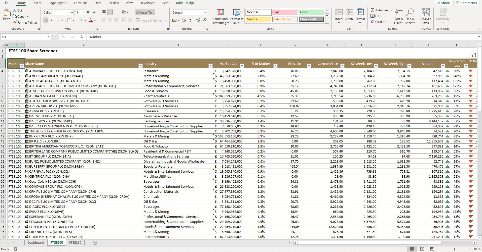
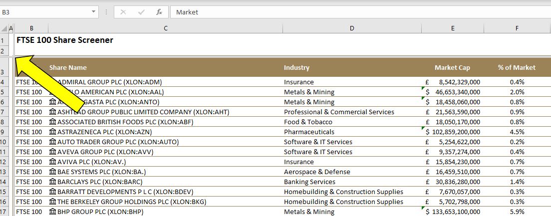
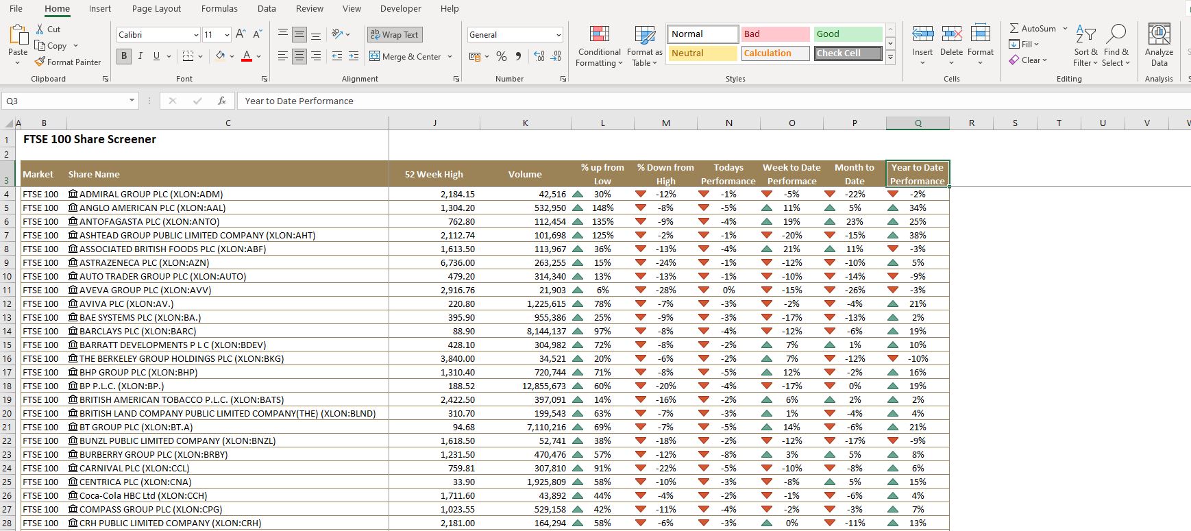
The below image shows a stock screening tool in Excel for the FTSE-100 index. This contains 100 rows of data (1 row per company) and has 16 columns of information ranging from the market name in column B to Year-to-date performance in column Q…
note column Q is currently off the visible screen area.
With so much information on display the user has no choice but to scroll down to find the companies towards the end of the range but the view they will be met with looks like this:
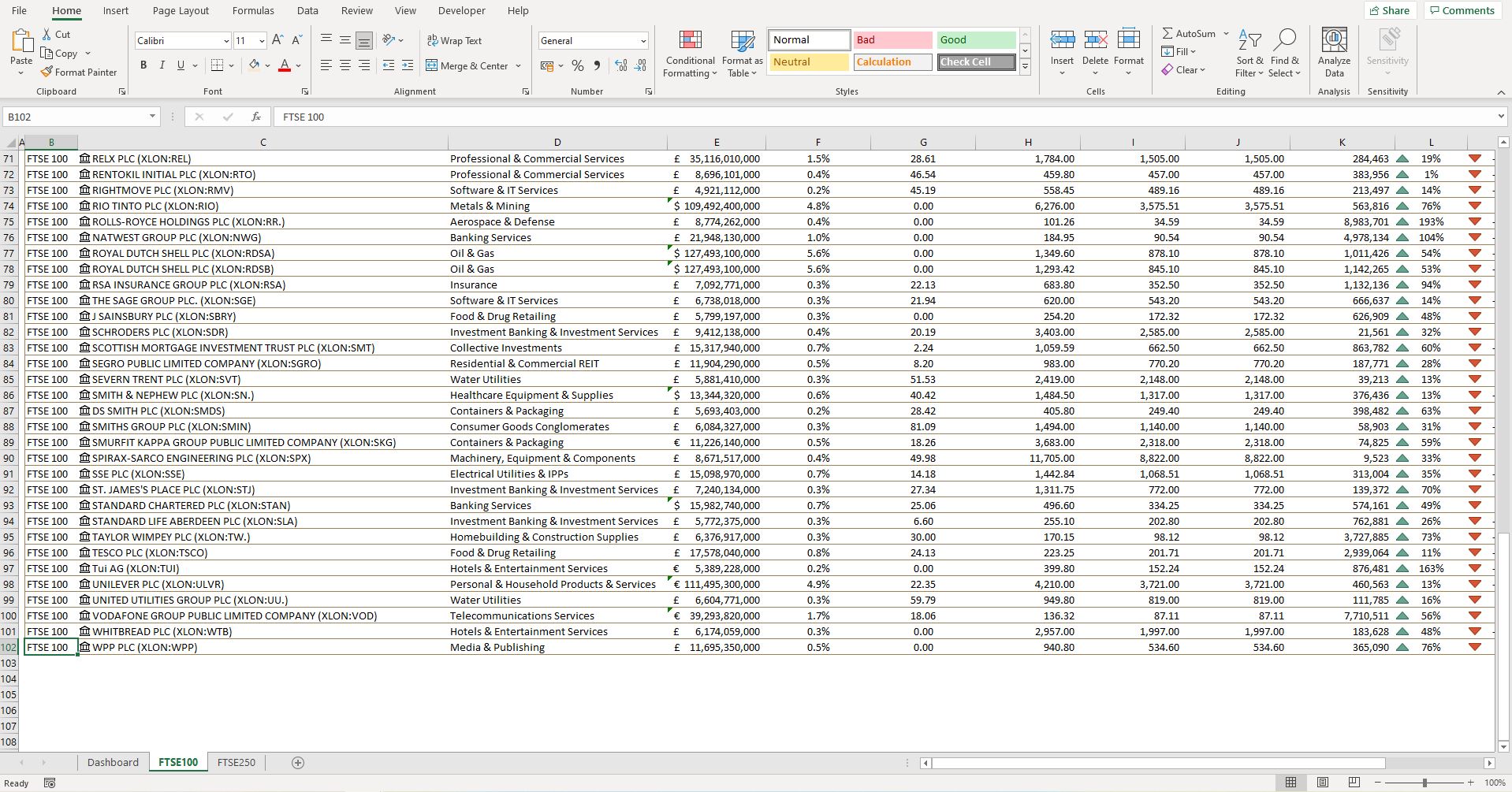
Can you remember what the data column G represents? Is that the price or the PE ratio? You can see that this view is not that user-friendly and it would be more helpful if the headings on row 3 were still visible.
Equally if the user scrolls across to column Q to see the year-to-date performance they will be met with a screen that looks like this:
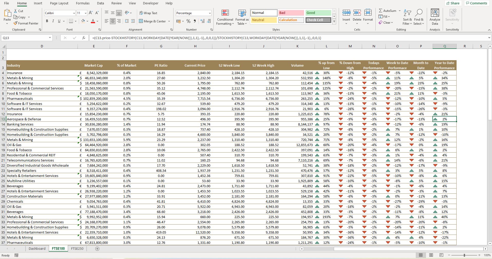
Now the user has no idea what company they are looking at as the share names are in column C which have disappeared off-screen by scrolling to the right.
Time to freeze some Excel panes and make this FTSE-100 stock screener more user-friendly.
Freeze Panes in Excel Solution
The first step as an Excel developer is to decide what has to be in view at all times. In this example there are two things that must be in view to make this worksheet user-friendly:
- The headings in Row 3
- The ‘Company Name’ in Column C
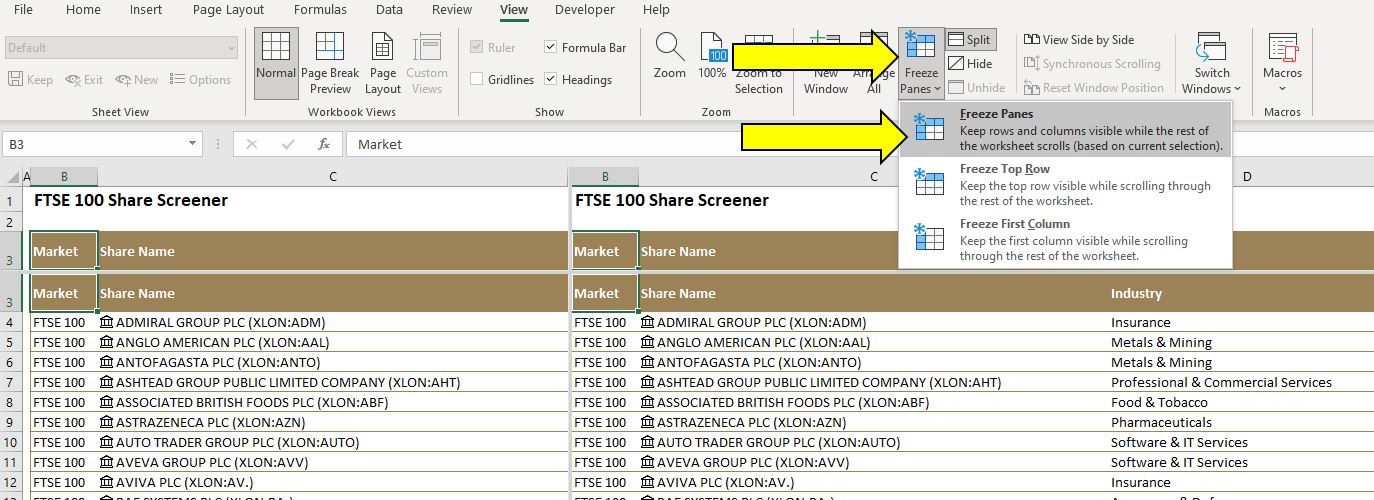
The first step is to select the ‘View’ tab from the Excel ribbon, followed by ‘Split‘ in the ‘Window‘ section:
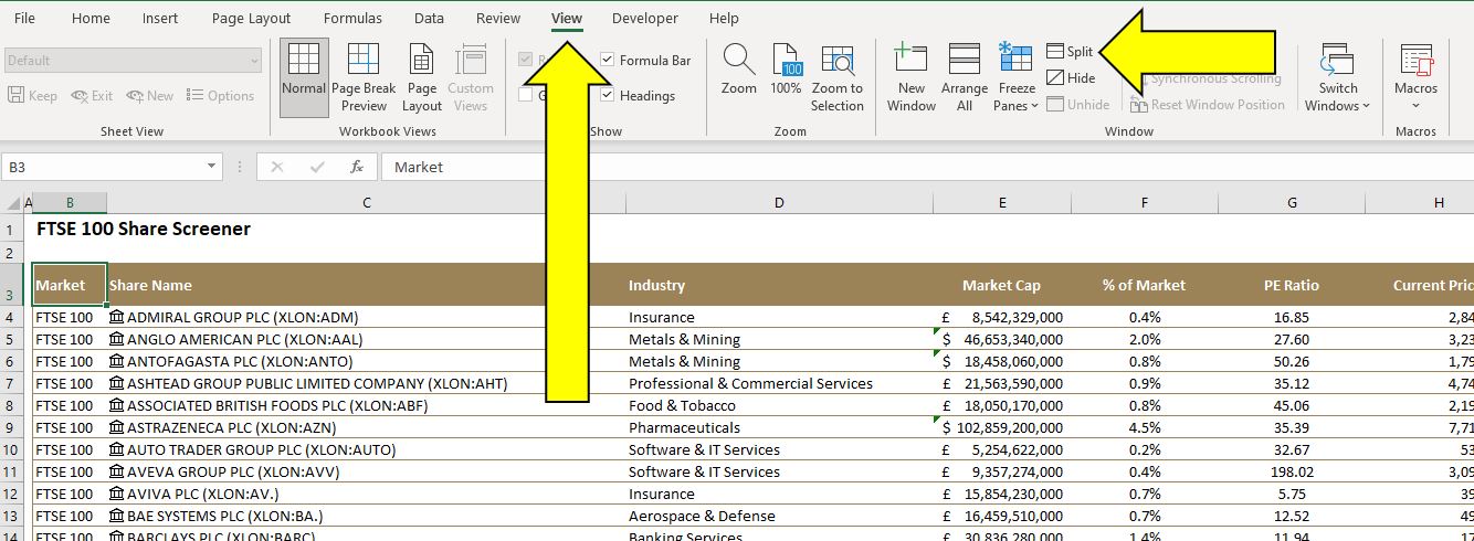
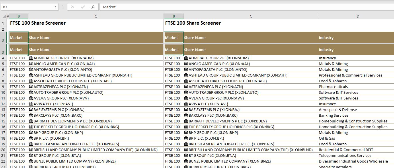
This activates the Split procedure and two moveable grey bars will appear on the worksheet, one horizontal and the other vertical. They can be a little difficult to see at first but if you look to the top left corner of the worksheet you will notice them intersecting:
Move the Excel cursor over the horizontal grey bar first. The cursor will change shape and then you can click on the grey bar to drag it below the headings. This is telling Excel to freeze everything above that line so in this case the headings.
Next drag the vertical grey bar so company name is to the left of it. Again this is telling Excel to freeze everything before that line, in this case it will capture the share name along with the market. The worksheet will look a bit odd as Excel duplicates the selections but this is a temporary view:
Finally go back to the Excel ribbon and click on the ‘Freeze Panes’ icon followed by ‘Freeze Panes’ from the menu that appears:
The process is complete and the panes have now been frozen in Excel.
The Results of Freezing Panes in Excel
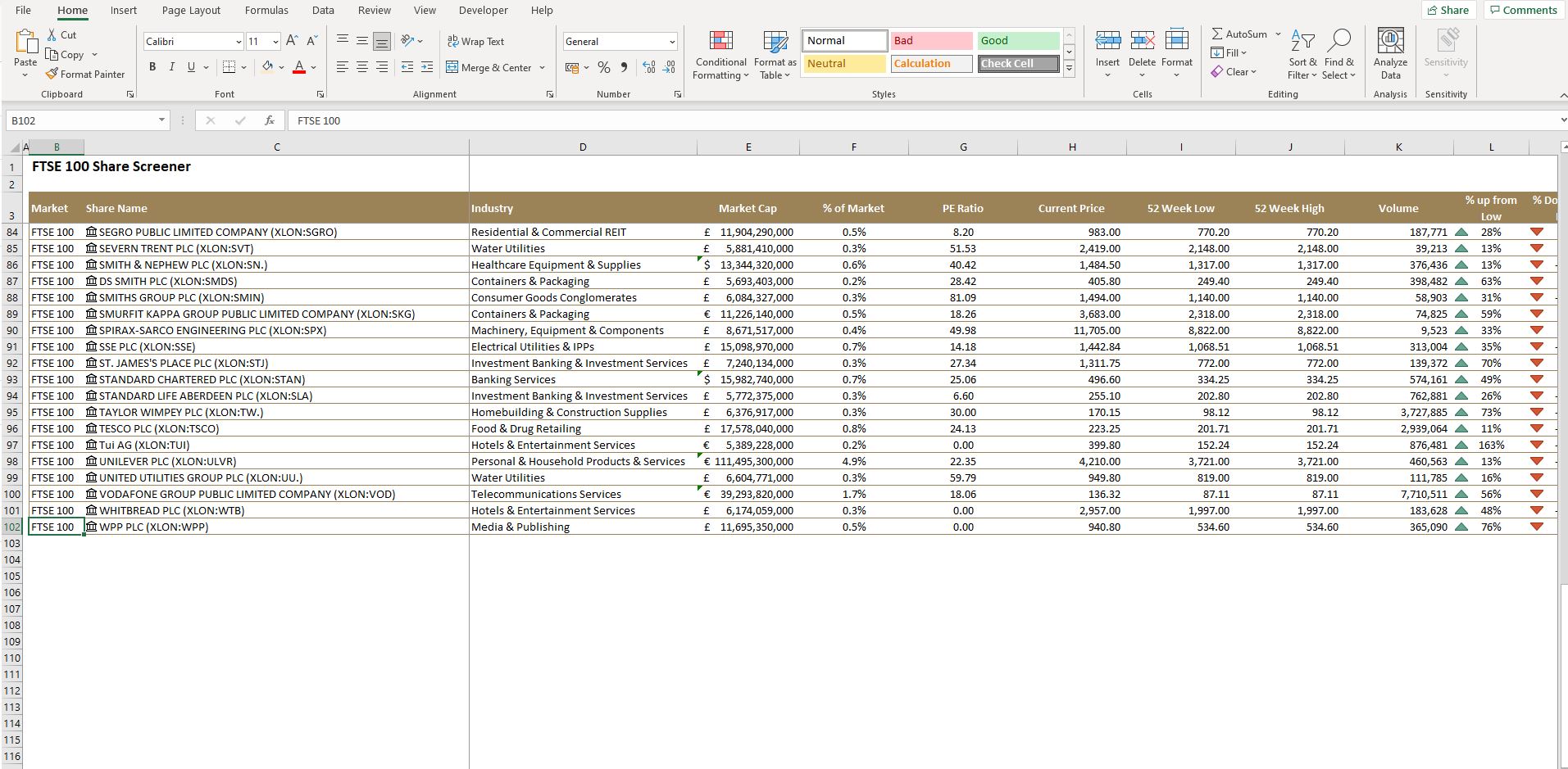
Now when the user scrolls to the bottom of the FTSE-100 Share screener they will be able to still see the headings:
Or if the user decides to scroll across to column Q and look at the year-to-date performance they will be able to see which share name they are looking at:
Tips for Freezing Panes in Excel
Freezing panes effectively in Excel can significantly enhance your data navigation experience. Here are some practical tips to get the most out of the freeze panes in Excel feature:
- Identify Key Data: Before freezing panes, determine which rows or columns contain essential data that you need to keep visible.
- Avoid Freezing Excessive Rows/Columns: Only freeze the necessary sections to maintain a clear view of your worksheet.
- Use in Combination with Split Panes: For even more control, consider using split panes along with freeze panes to divide your worksheet into more manageable sections.
- Test Different Scenarios: Experiment with freezing different rows and columns to find the most efficient layout for your specific dataset.
Remember, the goal of using freeze panes in Excel is to keep crucial data in sight at all times, enhancing your efficiency and accuracy in data analysis.
Conclusion
In summary, learning how to freeze panes in Excel is a powerful technique for anyone dealing with extensive datasets in their spreadsheets. By keeping important rows or columns constantly visible, you can navigate through large amounts of data with ease, ensuring no vital information is lost in the process. This guide has covered the essentials of how to freeze panes in Excel, along with practical tips to maximize its benefits.
Whether you’re working with financial reports, data analysis, or any other extensive Excel project, the ability to freeze panes is an indispensable skill that enhances both the usability and effectiveness of your spreadsheets. Embrace this feature to make your Excel experience more streamlined and productive.
Keep Excelling,

Ready to Add Even More Functionality to Your Excel Sheets?
After mastering how to freeze panes in Excel, why not take your skills up a notch? Dive into our next tutorial, “How to Assign Macros to Shapes,” and discover how to make your Excel worksheets not only visually engaging but also functionally interactive. Whether it’s streamlining tasks or adding a touch of creativity, this guide will show you how to transform simple shapes into powerful tools. Start enhancing your Excel projects with custom macros here!