
Mastering the VLOOKUP in Excel is a game-changer. This powerful function allows you to search through large datasets with precision and ease. Whether you’re consolidating information from various sources or seeking specific data points, understanding how to effectively use VLOOKUP in Excel can significantly enhance your spreadsheet capabilities.
Embark on this guide to unlock the full potential of VLOOKUP and elevate your Excel proficiency.
Understanding the VLOOKUP Function in Excel
The VLOOKUP function in Excel is an essential tool for efficient data retrieval. It follows the format:
- =VLOOKUP(Lookup_Value, Table_Array, Col_Index_Num, [Range_Lookup])
In this formula,
- ‘Lookup_Value‘ is the specific data you’re searching for within your table, like a unique identifier or reference number.
- ‘Table_Array‘ defines the range of cells where your data is located.
- ‘Col_Index_Num‘ specifies the column from which you want to extract the value.
- Lastly, ‘Range_Lookup‘ determines the match type: set it to FALSE for an exact match, which is often more useful, or TRUE for an approximate match.
For beginners in Excel, this might seem complex. However, in simpler terms, the VLOOKUP function tells Excel to “Find this value in a specified table, and return the corresponding value from a designated column.” An example will make this clearer.
VLOOKUP in Excel: A Practical Example
The best way to grasp the VLOOKUP function in Excel is through practical examples.
Here’s a straightforward scenario to help you understand its application. Remember, while this example uses a small dataset, VLOOKUP’s true power lies in its ability to handle much larger tables. The fundamental process of implementing a VLOOKUP in Excel remains consistent, regardless of the data size.
Example
If you would like to follow the example in Excel you can download the file here.
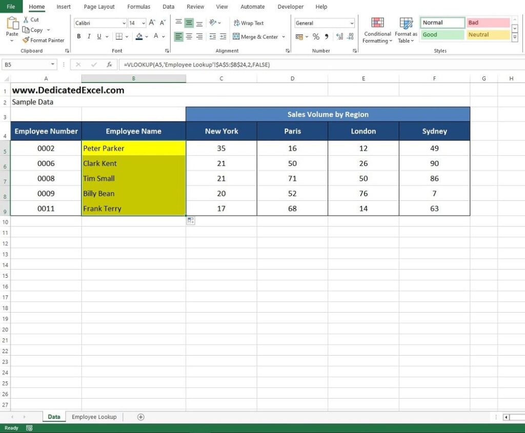
In the provided example, we have a table that details sales volumes by region for five employees within the company. The challenge arises from the fact that we only possess their employee numbers, while their names have not been recorded:
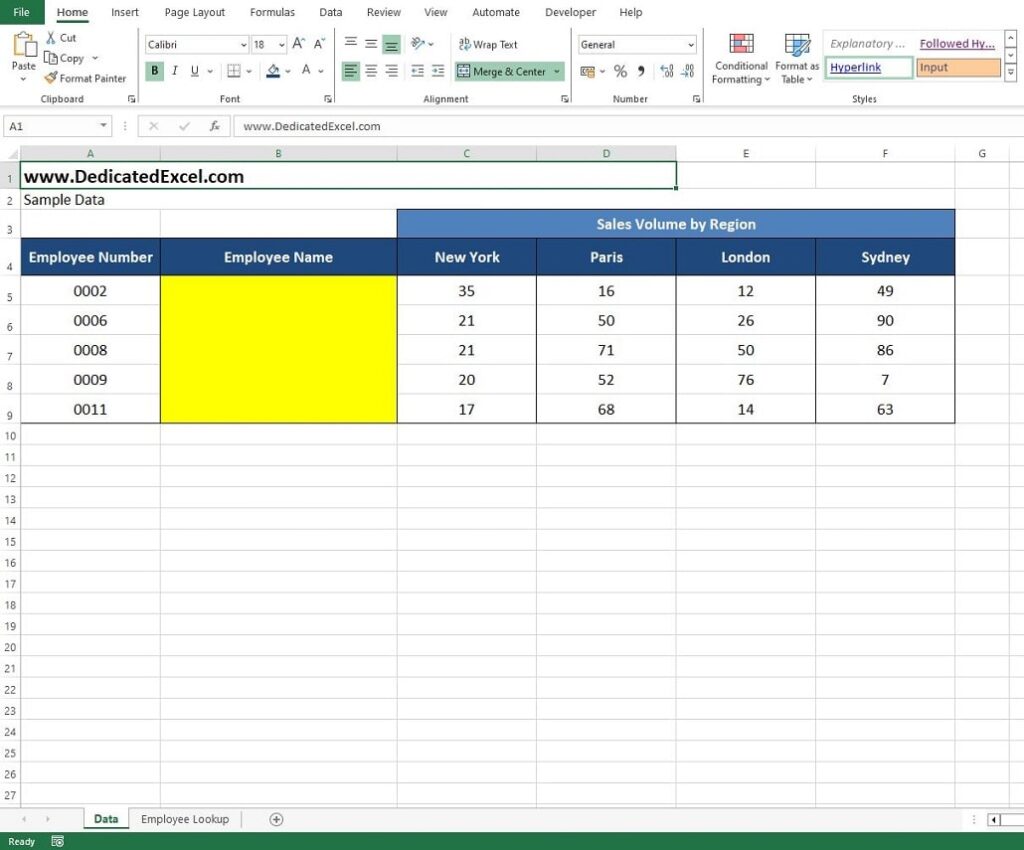
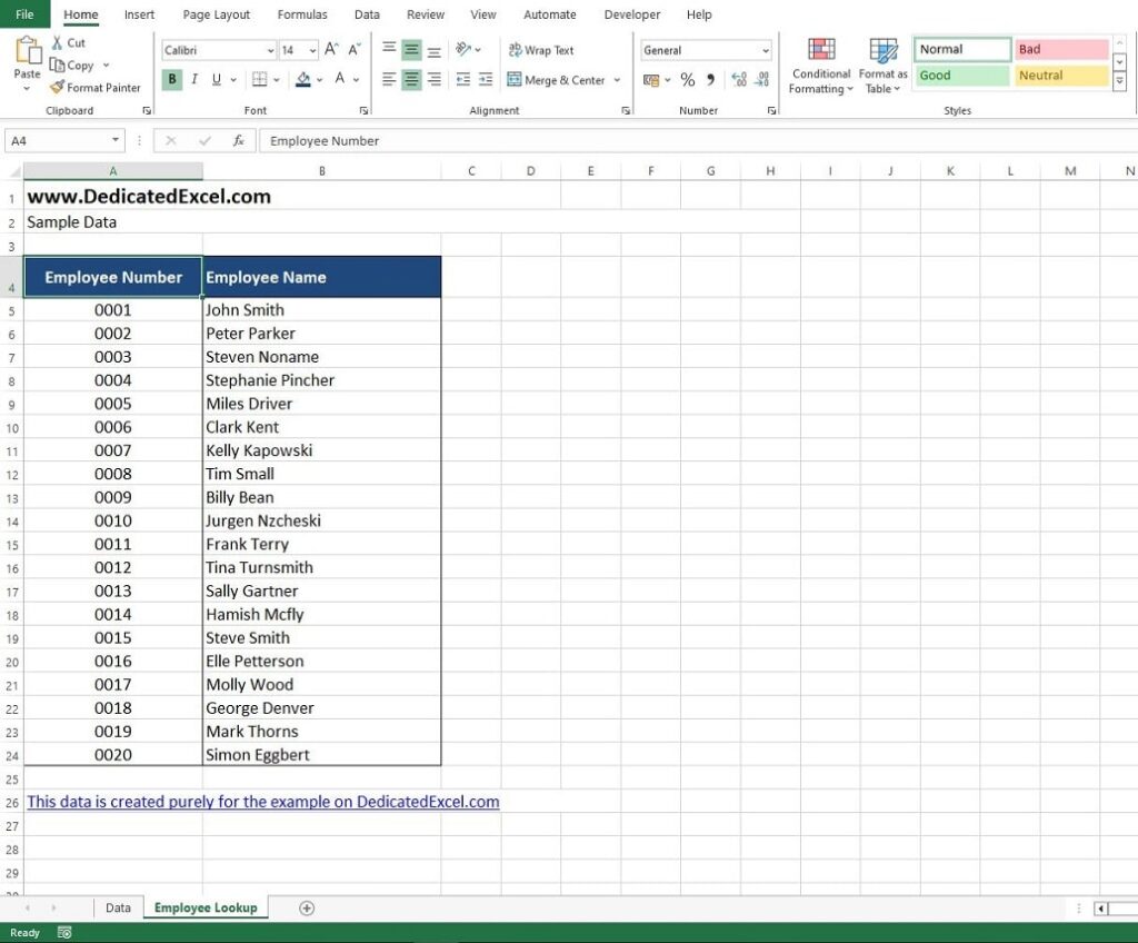
For the analysis, the employee numbers are insufficient. So, you contact the company’s Human Resources team, who provide you with a master list of all employees, including their employee numbers.
This comprehensive list, located on the ‘Employee Lookup‘ worksheet in the downloadable file, sets the stage for effectively utilising the VLOOKUP in Excel to match names with their corresponding employee numbers.
In this scenario, you are faced with two options.
The first is to manually sift through the lookup table to find the names of employees on your report.
The second, and far more efficient, method is to employ the VLOOKUP in Excel, which automates this process, eliminating manual labour. Automation, especially through formulas like VLOOKUP, is a best practice in Excel to ensure accuracy and save time.
Let’s revisit the structure of the VLOOKUP function in Excel:
- =VLOOKUP(Lookup_Value, Table_Array, Col_Index_Num, [Range_Lookup])
To apply this in our example, the following components are necessary:
- Lookup_Value: This is the employee number from your report. It serves as a unique identifier, and the goal is to match this number with the corresponding entry in the ‘Employee Lookup’ table.
- Table Array: The range of cells in the ‘Employee Lookup’ table. This tells Excel where to search for the employee number. It’s crucial to include all relevant columns in this range. In our case, both columns A and B are needed, as we require the employee’s name from the table.
- Col_Index_Num: Here, it will be 2, as the employee name is in the second column of our table.
- [Range_Lookup]: Set this to FALSE for an exact match, which is necessary to accurately pair employee numbers with names.
Implementing the VLOOKUP Function in Excel
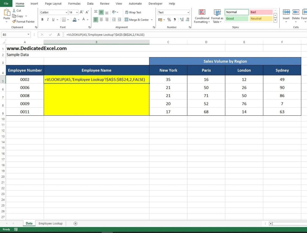
With a clear understanding of what you need and where to find it, you can construct the VLOOKUP formula. For instance, if the first employee number is in cell A5, begin there.
In cell B5, input the following:
- =VLOOKUP(A5, ‘Employee Lookup’!$A$4:$B$24, 2, FALSE)
Pay attention to the use of dollar signs ($) in the ‘Employee Lookup’!$A$4:$B$24 range. These ensure that the cell range remains fixed, allowing you to replicate the formula down the column of your report. Omitting these signs could lead to misalignment with the lookup table and potential errors.
Hence, the formula in cell B5 should appear as follows:
And the result should be Peter Parker, I guess it’s always handy to have Spider-Man working for the company!
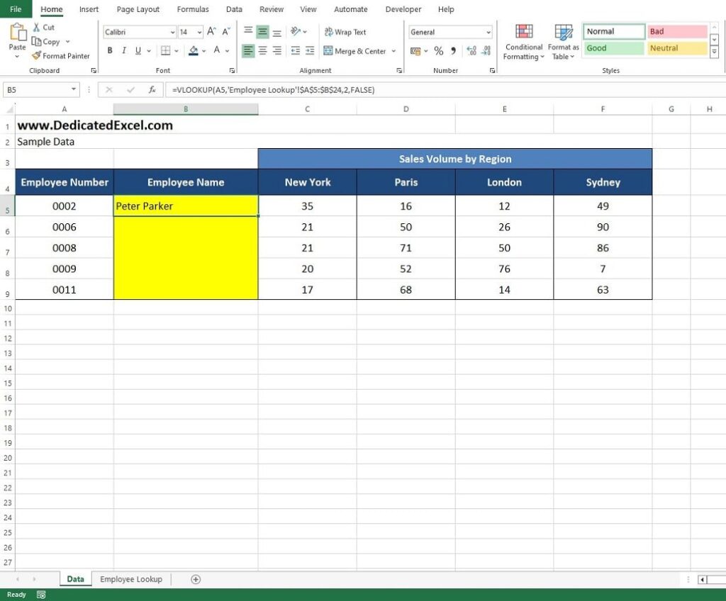
To finalise your report, replicate the formula for the remaining names. This can be done by selecting cell B5 and then dragging the fill handle from the bottom right corner of the cell down to B9.
This action will populate the table with the corresponding employee names, successfully achieving your goal of completing the report.
Summary
The example we’ve explored is just a glimpse into the robust capabilities of the VLOOKUP function in Excel.
At first glance, it may seem simpler to manually search for a few names, but the real strength of VLOOKUP becomes evident in more complex scenarios. When you’re dealing with reports that require referencing hundreds or thousands of records from expansive datasets, VLOOKUP in Excel emerges as an invaluable time-saving tool.
Its utility goes beyond just large-scale tasks; VLOOKUP is a versatile function that I’ve found indispensable in my extensive experience with Excel. It’s a skill that every proficient Excel analyst should master. By understanding and applying VLOOKUP in Excel, you’re not just performing tasks efficiently; you’re joining the ranks of advanced Excel users.
Welcome to the world of VLOOKUP – a club where data management meets efficiency and precision!
Keep Excelling,
Now that you’re adept at using VLOOKUP in Excel, take your skills further. Learn how to make an Excel Pivot Table update automatically for even smarter data management. Dive into our guide and transform your Excel expertise.