
Whether you’re an Excel novice or a seasoned spreadsheet wrangler, there’s a universal truth we all come to appreciate: the clearer your data presentation, the better. This is a straightforward guide to help you present negative numbers in red in Excel.
By learning how to display negative numbers in red in Excel, you’ll add a layer of instant, visual comprehension to your reports and dashboards. Let’s dive into this simple, yet impactful technique that will elevate your Excel skills and ensure your data speaks volumes.
Showing Negative Numbers in Red in Excel
Typically, the conventional wisdom in Excel reporting and dashboard design leans towards displaying negative numbers in red. This practice isn’t just for show; it serves a practical purpose. It offers an immediate, visual distinction between positive and negative values, an essential factor in ensuring clarity, particularly in densely-packed reports where every bit of readability counts. Unless specified otherwise by your client or manager, adopting this approach can significantly enhance the user’s ability to quickly interpret the data presented.
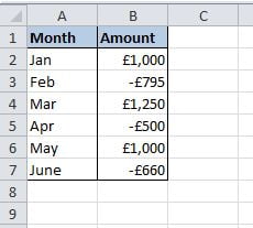
For example, this is the standard display:
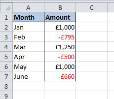
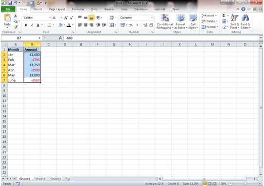
Now see the visual impact of displaying the negative numbers in red, they are much easier to identify:
How to Show Negative Numbers in Red in Excel
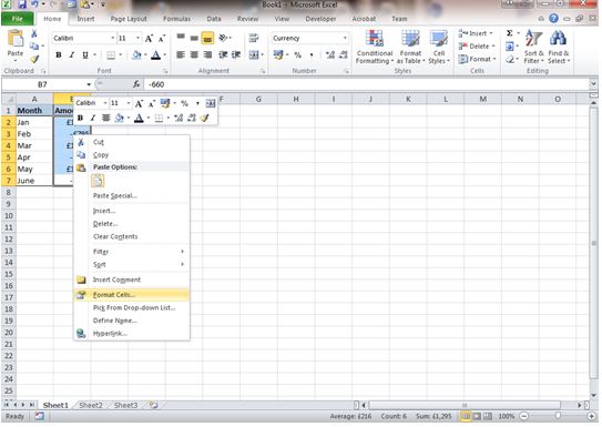
In order to show negative numbers in red in Excel the technique is simple, first off select the range of cells that you want to convert:

Next, right click on the selected area; from the pop-up menu select ‘Format Cells’.
For negative values the data must be numeric, which means selecting either ‘Number’ or ‘Currency’ from the Format Cells options box. For this example currency is selected:
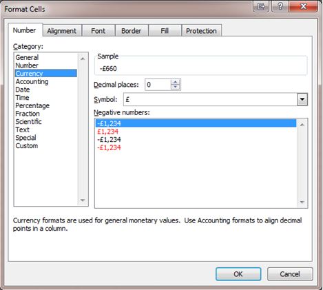
When you have selected either ‘Number‘ or ‘Currency‘ you can then choose how Excel will display the values. In order to make show negative numbers in red you need to select the correct option within the ‘Negative Numbers‘ category:
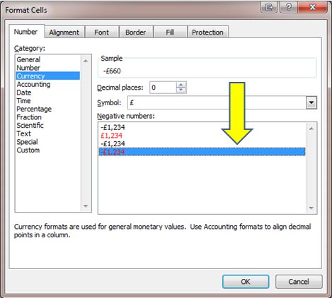
You will notice from the options in the ‘Negative numbers‘ section there are 2 unique ways of showing negative numbers as red in Excel, either with the minus sign in front of the number, i.e. -£100 or without the minus sign, i.e. £100.
Select a preferred choice then click “OK” and the values will update:
Now the negative values show as red in Excel and the process is complete.
It’s worth noting that the cells changed retain their new format so if you alter a positive to a negative in the range then that would also take the “red” formatting on.
Summary
In conclusion, displaying negative numbers in red in Excel is a simple yet powerful technique to enhance data clarity in your reports and dashboards.
By following the steps outlined in this guide, you can easily differentiate between positive and negative values, improving readability and efficiency in data analysis. Remember, this method not only aids in quick data interpretation but also adds a professional touch to your Excel projects.
Keep Excelling,

If you are ready for more Excel knowledge tips then check out these 5 time saving techniques for Excel – every Excel user should know them, do you?