
Exploring Excel Pivot Tables can initially seem daunting, especially for beginners. Whether you’ve faced challenges with these tables in the past or are encountering them for the first time, this guide is designed to demystify their basics.
Join us as we walk you through the fundamental concepts of Excel Pivot Tables, providing step-by-step instructions on how to create and utilize them effectively. This article aims to transform your approach to data analysis, making it simpler and more efficient.
Understanding the Excel Pivot Table?
An Excel Pivot Table is a powerful feature designed to simplify the way you view and interact with large sets of data. Imagine having a vast spreadsheet, like a record of sales transactions, and wanting to make sense of all that information quickly and easily.
A Pivot Table comes to your rescue by enabling you to create a condensed, organized table. This table not only looks more approachable but also allows you to interact with your data in meaningful ways.
When to use a Pivot Table in Excel
Imagine you have a spreadsheet filled with data – maybe it’s sales records, customer feedback, or a list of transactions – and you need a clear summary of this information. This is where an Excel Pivot Table becomes your go-to tool. It’s perfect for those moments when you need a quick, comprehensible overview of your data.
Pivot Tables are incredibly versatile and can handle datasets of various sizes. Whether it’s a few dozen entries or thousands, they work efficiently. However, when dealing with very large datasets, such as those over 100,000 records, you might face some practical challenges.
For example, if you need to share your file via email, the size could become an issue. This happens because a Pivot Table keeps the raw data within the file to stay functional and interactive, which naturally increases the file size. So, while Pivot Tables are excellent for summarizing large datasets, it’s good to be mindful of file sizes when sharing them.
How to create your first Pivot table
Creating a Pivot table is made easy in Excel, let’s jump into an example and show you how easy. If you want to follow along please download the dataset used in the example.
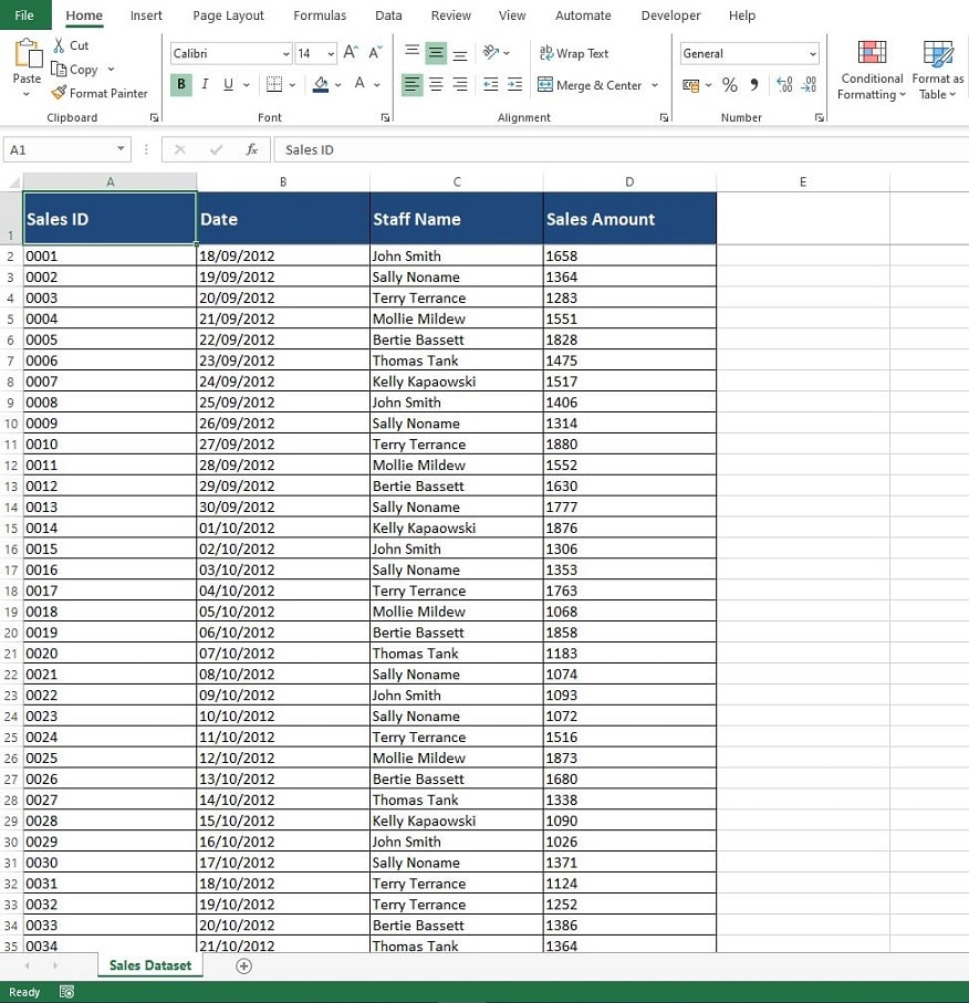
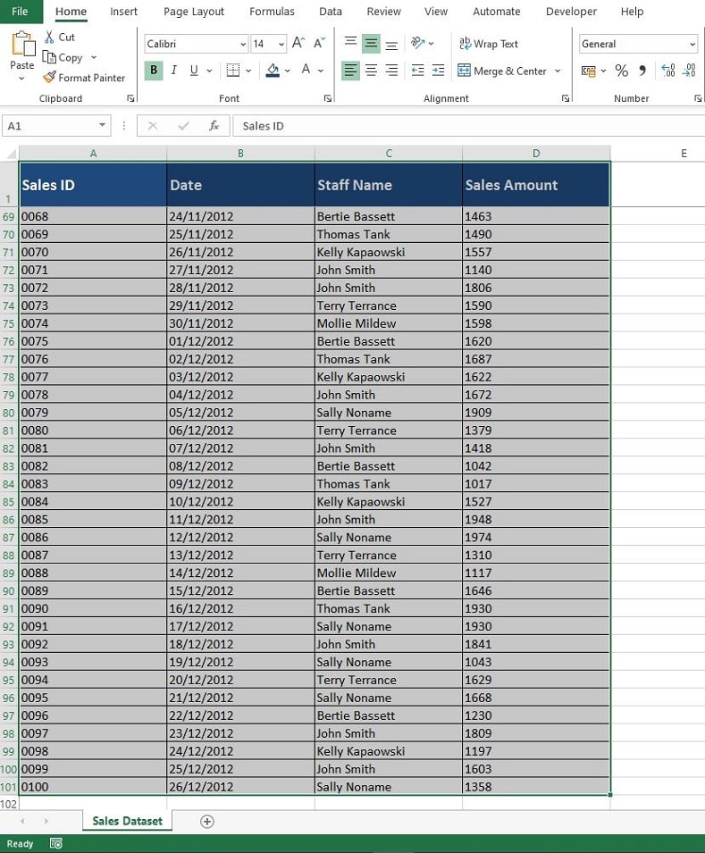
Highlight Your Data
The first step is to highlight the data range you want to include in your Pivot table, including the field headings. Remember, you can do this by clicking on the top left cell of your dataset, hold the left mouse button down, then drag the highlighted region across your entire dataset.
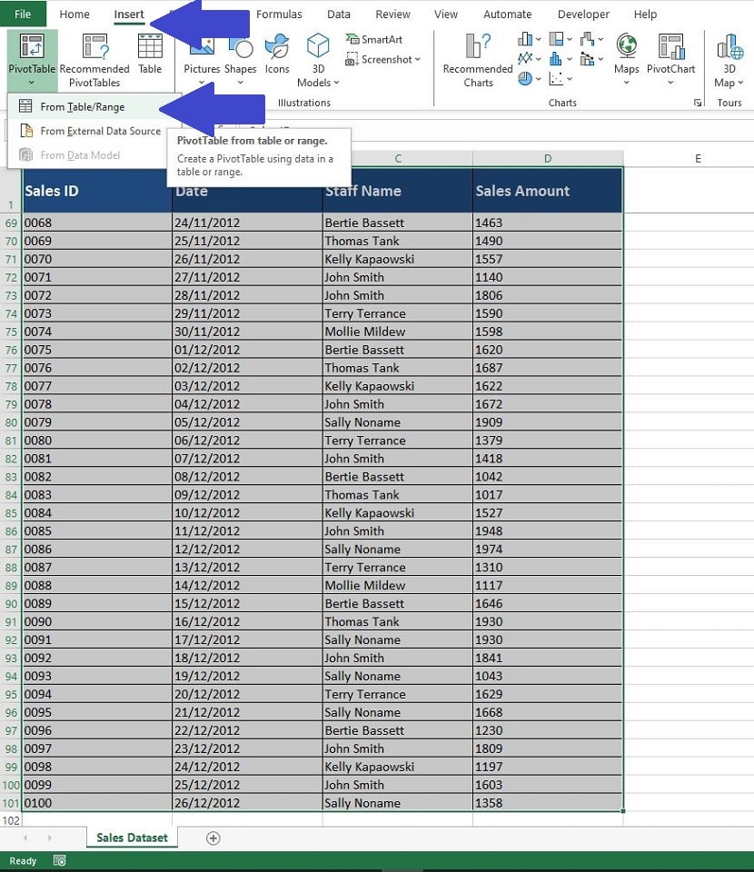
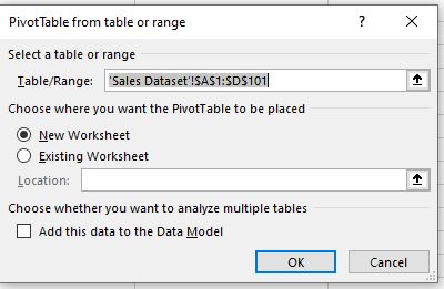
Insert the Pivot Table
With your data highlighted, click the ‘Insert‘ tab on the Excel Ribbon, then select ‘PivotTable‘ and select the first option, called ‘From Table/Range‘. You are then shown the ‘PivotTable from Table or Range‘ settings box, there is no need to change anything here as the data range has already been selected in the first step. Click ‘OK’ and you will be presented with your PivotTable Canvas.
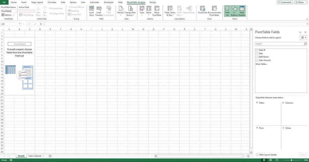
Populate the Pivot Table
Excel generates a blank Pivot table from your data range so the next step is to decide the layout of the Pivot table. On the right side of the worksheet you will see a new Excel pane called ‘PivotTable Fields‘, if you don’t see the pane then right-click on the blank Pivot table and select ‘Show Field List‘.
Drag the fields from the top section of the ‘PivotTable Fields‘ pane to the relevant Row, Column, Value and/or FIlters section.
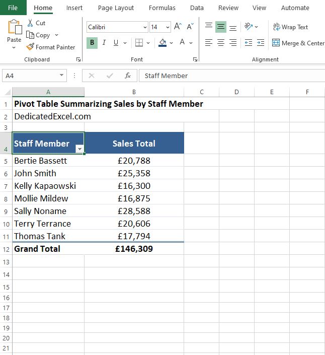
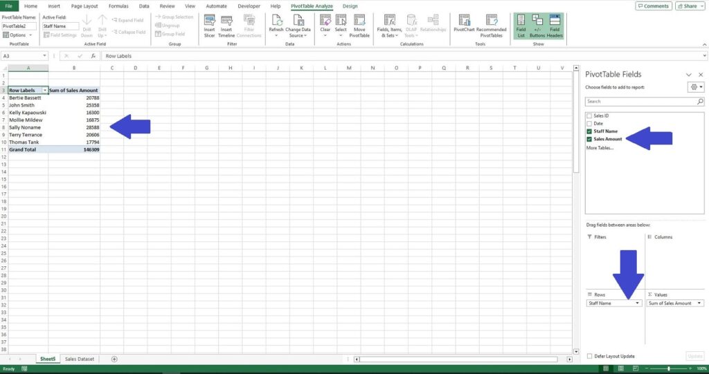
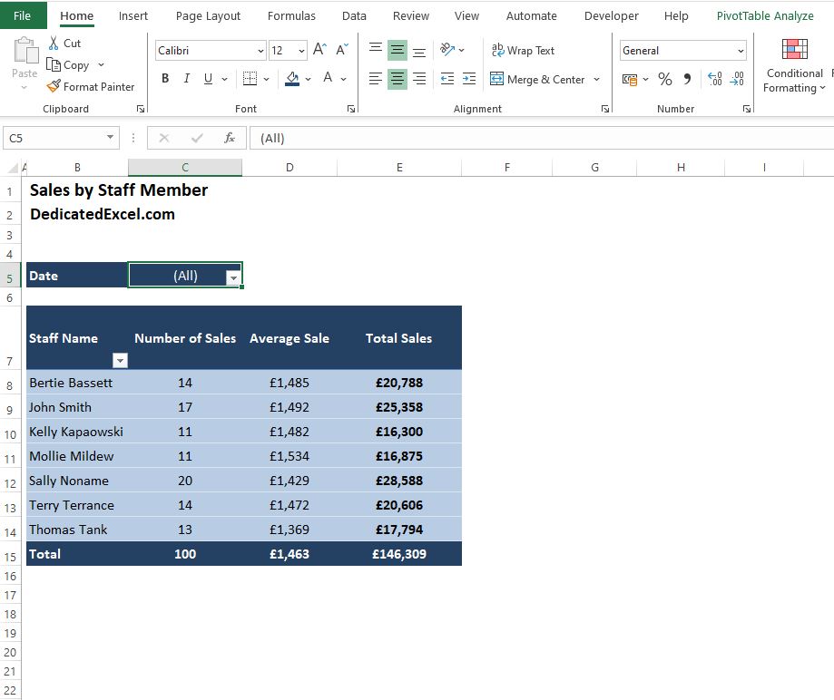
To create a basic Pivot table we can drag the ‘Staff Name‘ field to the ‘Rows‘ area and the ‘Sales Amount‘ field to the ‘Values’ area. This automatically creates a Pivot table on our Excel worksheet showing the Sum of Sales for each Staff Member.
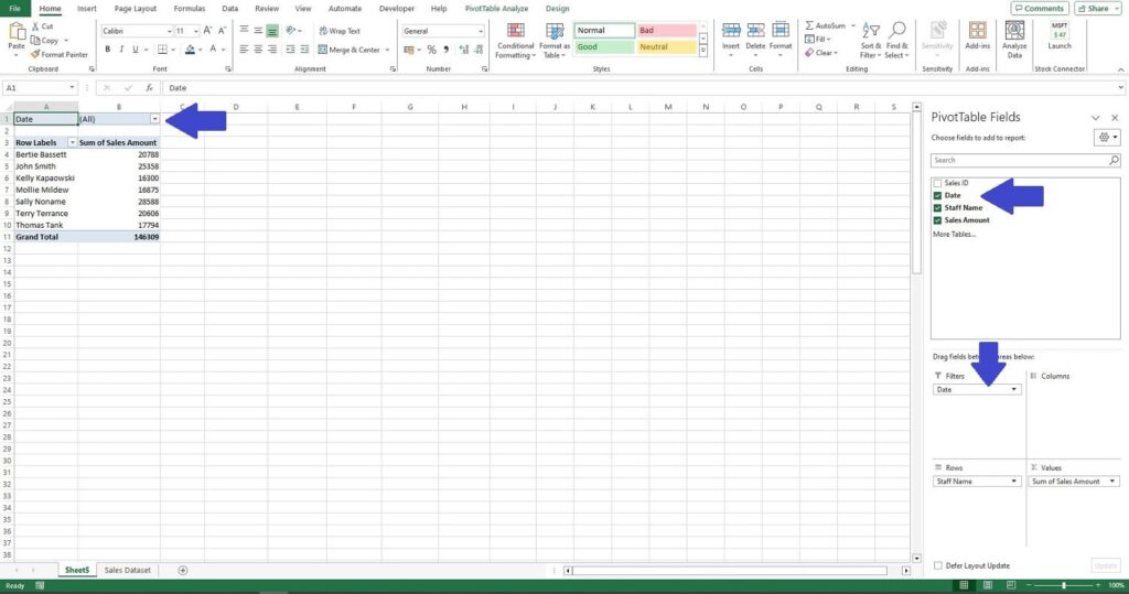
Add a Filter to the PIVOT Table
After the Pivot table is created, you can amend it at any time. For example, to include a filter for ‘Dates‘ on the previous table, click anywhere on the Pivot table to bring the ‘PivotTable Fields‘ pane back into view.
In the ‘PivotTable Fields‘ drag the ‘Date‘ field down to the ‘Filters’ area. You will see that the Pivot Table automatically updates to include the ‘Date‘ as a filter.
Customizing the PIVOT Table
Once you’ve created a Pivot Table in Excel, you’ll discover the joy of customizing it to suit your specific needs. Even as a beginner, you can easily make your Pivot Table more informative and visually appealing with a few simple tweaks. Here are some common and easy-to-implement customizations:
- Changing Number Formats: Often, you’ll want your data to display in a certain way, like showing currency, percentages, or just plain numbers. To do this, right-click on the data in your Pivot Table, select ‘Number Format,’ and choose the format that best suits your data.
- Switching Summaries from Sum to Average (or Other Functions): By default, Pivot Tables sum up your data. But what if you want to find the average instead? Just click on the drop-down arrow next to your value field, choose ‘Value Field Settings,’ and select ‘Average‘ or any other calculation method that fits your analysis.
- Adjusting the Colour Scheme: A dash of colour can make your data stand out. Excel offers a variety of colour schemes to make your Pivot Table more readable and visually appealing. You can access these by clicking on the Pivot Table and then selecting ‘PivotTable Styles‘ from the toolbar. Choose one that complements your data and the overall look of your report.
- Renaming Field Headers: Sometimes, the default field names in Pivot Tables aren’t very descriptive. You can change these to something more understandable by simply clicking on the field header in the Pivot Table and typing in a new name.
- Reorganizing Data: Drag and drop different fields between rows, columns, filters, and values areas to see different perspectives of your data. This flexibility allows you to explore and present your data in the most meaningful way.
Remember, the goal of customizing your Pivot Table is to make your data analysis as clear and impactful as possible. Start with these basic customizations, and you’ll see how your Pivot Table becomes not just a powerful tool, but also a reflection of your specific data needs.
Summary
In this guide, we’ve explored the versatile world of Excel Pivot Tables, a tool that’s both powerful and accessible, especially for beginners. From understanding what a Pivot Table is and recognizing its immense value in summarizing and analysing large datasets, to the step-by-step process of creating and customizing your own Pivot Table, we’ve covered the essentials to get you started.
Pivot Tables are more than just a feature in Excel; they are a gateway to efficient data management. By learning how to create, edit, and customize these tables, you’re not only improving your Excel skills but also gaining a valuable asset in your data analysis toolkit. The ability to quickly transform complex data into clear, concise, and visually appealing summaries is a skill that will serve you well in any data-driven task.
As you continue to explore and experiment with Pivot Tables, remember that practice is key. Don’t hesitate to try different customizations or explore various ways of presenting your data. Each dataset offers a new opportunity to discover the potential of Pivot Tables.
Keep Excelling,

Ready to Level Up Your Pivot Table Skills? Next, discover how to make your Excel Pivot Table update automatically! This essential follow-up guide will show you the steps to ensure your data stays fresh and accurate, saving you time and effort. Read our next article: How to Make an Excel Pivot Table Update Automatically and keep your data analysis game strong!