Have you ever needed the most recent data point in a complex Excel row? Mastering the ‘Last Value in a Row Excel’ technique is your key to success. Whether you’re building comprehensive dashboards or automating routine reports, this skill is essential.
In this guide, I’ll walk you through a straightforward approach to easily locate the last value in any row, enhancing your Excel toolkit. Ready to streamline your data processes and keep your analyses up-to-date? Let’s dive in and discover how to make Excel work smarter for you.
What Does Finding the Last Value in a Row Mean?
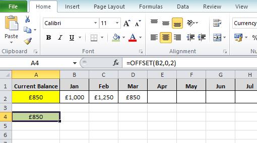
Lets set the background for clarity. In the example Excel spreadsheet table below there are a series of monthly balances. The monthly balances are captured in row 2.
In cell A2 is where the Current Balance is displayed. For this example we want this to always show the last value in row 2, because that is the most recent balance:

How to Find the Last Value in a Row of Data
To achieve our goal we need to create a “Last Value in a row Excel formula”
To do this we can create an Excel formula that utilises the OFFSET and MATCH functions.
- The OFFSET function is like a navigator, allowing us to move across a row from a specific starting cell. In this case, it helps us traverse along row
- The MATCH function is like a detective, designed to search for a specific item within a row and tell us its position.
By cleverly combining OFFSET and MATCH, we can pinpoint the exact location of the last value in a row, making this technique extremely useful for efficiently managing and analysing data in Excel.
Formula to Find the Last Value in a Row
In terms of the example the formula you would enter into cell A2 on the spreadsheet is:
=OFFSET(B2,0,MATCH(MAX(B2:XFD2)+1,B2:XFD2,1)-1)
By doing so the last value in row 2, which is currently £850 in March, is displayed:

The formula means that next month, when April’s balance is updated, the current balance will automatically reflect the change and show the balance as £1,100 for April:

How the Formula Works
Now that we have created our Last Value in a row Excel formula let’s delve into a more comprehensive exploration of the OFFSET and MATCH functions. Gaining a nuanced understanding of these two essential Excel functions is invaluable.
Not only does it bolster your confidence in crafting and devising bespoke Excel solutions, but it also equips you with the expertise to navigate complex data sets with ease. Understanding the mechanics of OFFSET and MATCH is a cornerstone for any Excel user looking to elevate their data analysis and reporting capabilities.
OFFSET Function in Excel
The OFFSET function in Excel is a versatile tool for navigating through your worksheet. It uses the formula structure =OFFSET(Reference, Rows, Columns), where ‘Reference’ is your starting cell, and ‘Rows’ and ‘Columns’ specify the movement from this point.
Take our ‘Current Balance’ example: by entering =OFFSET(B2,0,2), we instruct Excel to begin at Cell B2, then move 0 rows down and 2 columns to the right. The result is £850, as shown in the accompanying image.

However, OFFSET alone isn’t sufficient for dynamically locating the last value in a row of data. This limitation arises because you would have to manually update the formula each month to shift across an additional column.
To overcome this, we integrate the MATCH function, which complements OFFSET by automating the column traversal based on specific data conditions in your Excel sheet.
MATCH Function in Excel
The MATCH function in Excel is designed for precision in data searching. It follows the format =MATCH(Lookup Value, Lookup Array, [Match Type]).
In our scenario where we created the last value in a row Excel formula, we use a clever technique: we instruct Excel to locate the highest value in a row, then add 1. This sum becomes our ‘Lookup Value’. Our ‘Lookup Array’ spans all cells in row 2 from column B. The ‘Match Type’ is set to 1, meaning the function searches for values less than the lookup value.
Consider the isolated MATCH part of our formula. In our example, it returns the number 3 for three columns of data. This result occurs because Excel identifies the maximum value in row 2 (£1250), increments it by 1, and then counts the number of values below £1251, equating to three in this instance.

Importantly, the MATCH function dynamically adapts to additional data or even blank entries. Therefore, even if a month’s data is missing, it reliably locates the last column with data from B2 onwards.
This adaptive capability makes MATCH an ideal partner for the OFFSET function, together providing a robust solution for navigating and analysing Excel data.

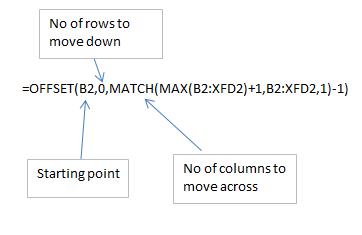
Combining the two, this is how the MATCH function then forms the columns part of the original OFFSET:

Summary
In summary, mastering the ‘Last Value in a Row Excel’ technique using the OFFSET and MATCH functions is a pivotal skill for anyone looking to elevate their Excel proficiency.
As we’ve explored, OFFSET allows us to deftly navigate across rows, while MATCH provides the precision needed to locate specific data points. By combining these functions, we unlock a powerful method for dynamic data analysis and reporting. Whether you’re creating detailed dashboards or automating routine tasks, this technique ensures your data is not only accurate but also effortlessly up-to-date.
Embrace these functions to transform how you interact with Excel, making your data work smarter for you.
Time to learn more great Excel tips? Progress to the next level and learn how to lookup a value in Excel based off the row and column and get a deeper understanding of Excels OFFSET and MATCH functions.


