The ability to lookup a value in Excel based off the row and column is a fundamental skill that elevates your Excel data analysis to new heights. In this guide, we demystify the process using Excel’s index and match functions.
Whether you’re reconciling data, extracting specific details, or simply streamlining your workflow, understanding how to effectively lookup values based on both row and column criteria is a valuable asset.
Jumping Right In
Lets jump right into performing a task in which we need to lookup a value in Excel based off the row and column. You can download the Excel file here if you want to follow along with the example.
Example
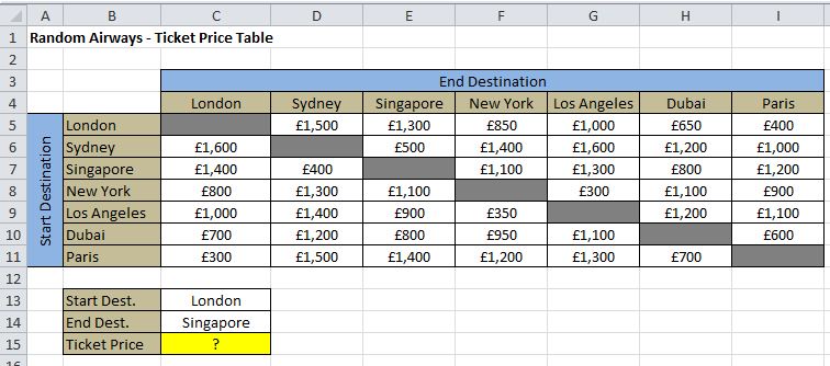
Your client emails you the following spreadsheet containing ticket prices for various flights at Random Airways, she wants to be able to enter the start destination and the end destination and for Excel to return the ticket price from that table, pretty nifty:

As an adept Excel analyst, you’ll recognize that this task involves aligning a starting and an ending destination, with the aim of retrieving a value based on these two points.
In Excel terms, this process entails identifying a specific row number and a column number, and then pinpointing the intersecting value at their junction. This intersection, or the ‘intercept’, is the focal point where the desired data resides. In basic terms we need to lookup a value in Excel based off the row and column
The Solution to looking up a value based on the row and column
Solving the task of ‘looking up a value based on the row and column’ in Excel requires a strategic approach. Start by breaking down the task into manageable segments – a technique equally effective for intricate IF statements. This problem can be dissected into three key steps:
- Identifying the row containing the start destination.
- Locating the column with the end destination.
- Retrieving the value at the intersection of these start and end points.
By methodically addressing each segment, you streamline the process, ensuring a precise and efficient solution to this Excel challenge.
Part 1 – Identifying the row containing the start destination
The first step in our journey to lookup a value in Excel based off the row and column is to identify the row with the start destination. For this, the MATCH function is our go-to tool.
Its syntax is: =MATCH(lookup_value, lookup_array, [match_type]).
Here, lookup_value is the value or cell reference you’re searching for. Lookup_array is the range B5:B11 in our example, encompassing all potential start destinations. We use match_type set to zero for an exact match.
In practice, our formula looks like =MATCH(C13,B5:B11,0).
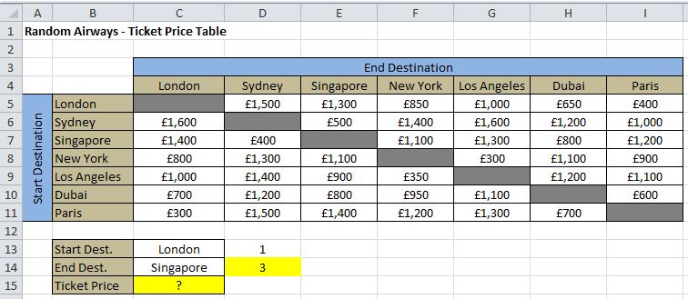
Applied to cell D13, it correctly identifies ‘London‘ as the first row in our range, returning the result ‘1‘. This precise identification is crucial for accurately finding our intersecting value later in the process.

Part 2 – Locating the column with the end destination
To pinpoint the column housing our end destination, we can again leverage the MATCH function for its efficient cell position identification.
In this scenario:
- ‘lookup_value’ is specified as the end destination in cell C14.
- ‘Lookup_array’ is defined from C4:I4, encompassing all end destination options.
- ‘Match_type’ remains zero to ensure an exact match.
Using the formula =Match(C14,C4:I4,0) in cell D14, we confirm our result. The formula outputs ‘3‘, indicating that Singapore, our end destination, is positioned in the third column of our range, a crucial step in our data analysis process.

Part 3 – Retrieving the value at the intersection of these start and end points
The final step in our Excel task is to retrieve the value where the identified row and column intersect. For this, the INDEX function is our solution. It’s structured as =INDEX(array, row_num, [Column_number]), where ‘array’ is the cell range, ‘row_num’ is the identified row, and ‘column_number’ is the found column.
In our example:
- ‘array’ is C5:I11.
- ‘row_num’ comes from Part 1’s MATCH formula (=Match(C13,B5:B11,0)).
- ‘column_number’ is from Part 2’s MATCH formula (=Match(C14,C4:I4,0)).
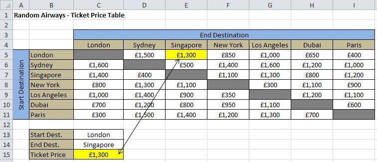
Combining these, the final formula =INDEX(C5:I11,MATCH(C13,B5:B11,0),MATCH(C14,C4:I4,0)), when entered in C15, reveals that the cost from London to Singapore is £1,300. This value aligns perfectly with our data table, confirming the accuracy of our approach.
Summary
Now that you have hone through the example of how to lookup a value in Excel based off the row and column you can see that efficiently navigating Excel often involves this task. For such scenarios, the combination of Excel’s INDEX and MATCH functions proves to be invaluable.
The key lies in breaking down the task into manageable parts: first identifying the row and column, and then integrating these findings into the INDEX function. It’s crucial to test each component for accuracy before combining them.
This step-by-step approach not only simplifies the process but also ensures precision in your results. With practice, mastering this method to effectively lookup values will become an intuitive part of your Excel toolkit.
You can download a copy of the completed example in Excel, with working formula here.
Keep Excelling,

Kudos on expanding your knowledge today – you’re definitely making strides! Now, let’s add an exciting twist to your learning journey: ‘how to get crypto prices in Excel‘. This skill isn’t just about crunching numbers; it’s a gateway to the dynamic world of cryptocurrency. Imagine tracking Bitcoin, Ethereum, and other cryptos in real-time, right from your Excel spreadsheet. Could this be your stepping stone to becoming a savvy crypto investor? Grab this opportunity to turn your Excel skills into a financial superpower!


