
Discover the art of dynamic Excel reporting and dashboard creation by learning how to manipulate Pivot Table filters through cell references using VBA. This technique is not just a skill, but a gateway to elevating your Excel proficiency into the realm of elite analysis.
Join me and delve into this invaluable method, enhancing your toolkit for customized reporting and data visualization.
Introduction
An Excel Pivot table filter is usually controlled and changed by the user who will select their option(s) using the Pivot tables drop down list on the filter:
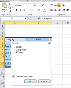
Using this drop down list and selecting your filter category is a simple enough task but when building user-friendly reports or Excel dashboards you might find it useful to change the pivot table filter, or more commonly numerous pivot table filters, on behalf of the user when they just change a single cell reference on the worksheet.
How to Create a Cell Controlled Pivot Table with VBA
The best way to show how the customization works in practice is to complete a simple example, once you have grasped the basic concept it can be embellished into something vastly more complicated.
First you need some data and a PIVOT Table. If you have your own data you can work through the example using that, alternatively if you want to follow this exact example through you can download the file here.
Background to the Download File
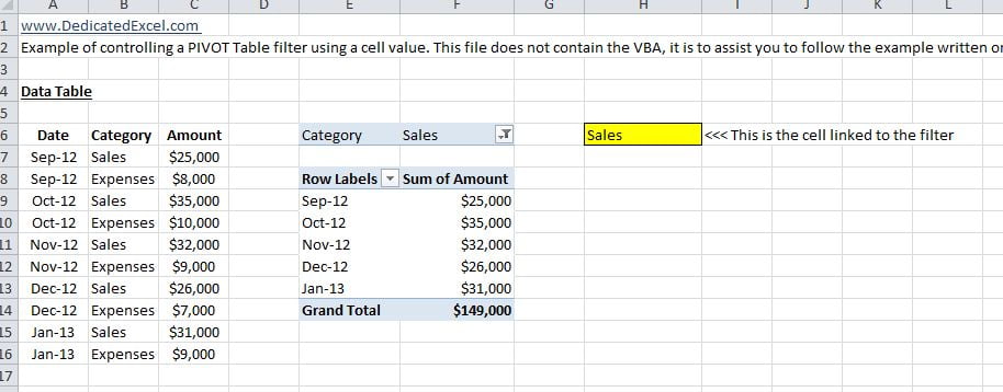
This file contains financial amounts (Amount) of sales and expenses (Category), by month (Date).
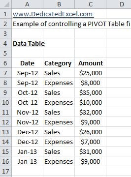
The aim is to have the pivot table show either Sales or Expenses depending on the value in a cell.
Step 1 – Identify the cell that you are going to use to contain the filter value
In this example cell H6 is used.
This cell will ultimately contain the text “Sales” or “Expenses” and depending on what text is in the cell that is what the PIVOT table filter will change to show.
Step 2 – Add the VBA for controlling the PIVOT table filter from the cell reference
To achieve any kind of update when a cell changes the VBA must be as a worksheet change script.
- The first action is to open up the VBA editor. Do so using the shortcut command (ALT+F11) or via the ribbon by selecting Developer then Visual Basic.
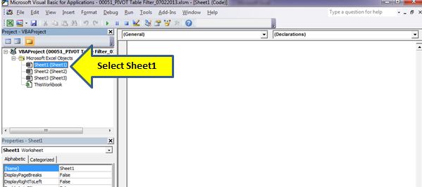
- The second action is to select the worksheet that the change is going to occur on. The aim is for the PIVOT table to update when the user changes the text value in Cell H6, this is on ‘Sheet1‘ of the example file so in the VBA Project explorer (upper left of the VBA window) select Sheet1:
- Now the correct sheet has been selected it’s time to let Excel know that this is a worksheet selection change script. To do so change the object drop down from its current state (General) to Worksheet. Upon doing so you will see some initial VBA script appear in the code window and the procedure drop down box (to the right) will automatically change to SelectionChange:
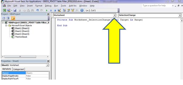
- Excel now knows that this VBA script applies to a selection change on the Worksheet, Sheet1 – it’s time to write the script that will update the PIVOT table.
For the readers looking for just VBA script I have place the full script below, you can just copy and paste this into your code window and save before moving onto the next step. If you want to get into more detail there is more explanation by reading on from here.
The VBA Script
Private Sub Worksheet_SelectionChange(ByVal Target As Range)

'This line stops the worksheet updating on every change, it only updates when cell
'H6 or H7 is touched
If Intersect(Target, Range("H6:H7")) Is Nothing Then Exit Sub

'Set the Variables to be used
Dim pt As PivotTable
Dim Field As PivotField
Dim NewCat As String

'Here you amend to suit your data
Set pt = Worksheets("Sheet1").PivotTables("PivotTable1")
Set Field = pt.PivotFields("Category")
NewCat = Worksheets("Sheet1").Range("H6").Value

'This updates and refreshes the PIVOT table
With pt
Field.ClearAllFilters
Field.CurrentPage = NewCat
pt.RefreshTable
End With

End Sub
The VBA Explained
Going through each section of the VBA script:
- If Intersect(Target, Range(“H6:H7”)) Is Nothing Then Exit Sub
In terms of this example a worksheet change means that whenever ANY change is made on Sheet1 Excel will refresh the pivot table. In reality we only want Excel to refresh the table when H6 is changed.
This code tells Excel that it should only action the worksheet change script when either H6 or H7 is touched. Why H7 when the key value is in H6? Because when the user types in “Sales” or “Expenses” they will usually follow that by hitting the ENTER key which will move the cell selection to down to H7, so we want that movement to trigger the change script.
- Dim pt As PivotTable
- Dim Field As PivotField
- Dim NewCat As String
This code enables us to refer to a Pivot table as pt, a Pivot field as Field and the cell reference H6 as NewCat. This is more about good practice in VBA writing as using shorter reference fields makes the remainder of the code cleaner and more user-friendly for error checking and debugging.
- Set pt = Worksheets(“Sheet1”).PivotTables(“PivotTable1”)
- Set Field = pt.PivotFields(“Category”)
- NewCat = Worksheets(“Sheet1”).Range(“H6”).Value
This code tells Excel what the variables pt, Field and NewCat refer to in this instance. If you are following your own example then you need to change this part to relate to your data as this is all file specific.
For the example used on this post pt is PivotTable1 on Sheet1, Field is the name of the filter being changed so that is “Category” and NewCat, the new value of the category, can be found in the cell H6.
- With pt
- Field.ClearAllFilters
- Field.CurrentPage = NewCat
- pt.RefreshTable
- End With
Finally this code tells Excel what action to take, this is the bit making the pivot table change. The first line “With pt” tells Excel the following code applies to the pivot table, PivotTable1 on Sheet1 (see previous section where we set the value for pt).
The next line “Field.ClearAllFilters” is to clear the current filter in place, then the third line, “Field.CurrentPage = NewCat” tells Excel to replace the filter with the value NewCat (which is the value in cell H6), then to close we tell Excel to refresh the pivot table pt and end the statement.
Completing the Example
- With the VBA script added it is time to save the file. Make sure that the file is saved as a “Macro Enabled Workbook” otherwise the changes will not work.
- The example is now complete. If the steps have been followed correctly the change can now be seen in action. If you change cell H6 to “Sales” and hit the enter key the pivot table will update to the Sales category:
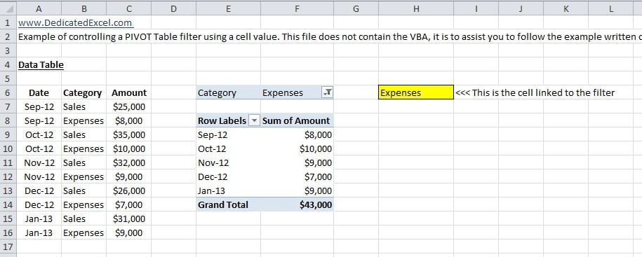
Or if you change the cell H6 to “Expenses” you will get an Expenses view of the data:
Download a working version of the final example click here.
Summary
To most Excel analysts this will seem like a lot of effort just to change the filter on a PIVOT table, especially when you can tell even the most non-technical user to use the existing drop down filter on the PIVOT table. However, the more important thing to grasp in this example is the concept of what is being achieved and realise the benefits on large scale Excel reporting.
Working on custom reporting solutions or Excel dashboards it is possible to have situations where there can be 10, 20 or (Insert large number here!) amount of pivot tables in a report and having the ability to control and update all the filters from 1 cell is very beneficial.
A practical and common example of this is where a report is created for multiple teams in a business.
Using this method it is possible to create one dashboard or report for all the teams and by simply changing 1 cell value they can see all the PIVOT tables in that report refresh just for their specific team, that’s a huge time-saver, a neat feature and ensures accuracy throughout the business as people can easily forget to change a filter when the report has lots of them.
Keep Excelling,

Are IF formulas in Excel leaving you puzzled? If so, check out our latest post, ‘How to Become an IF Formula in Excel Expert.’ We’ll guide you through the complexities of IF formulas, turning confusion into clarity and making you an Excel whiz in no time. Dive in for expert tips, practical examples, and the secrets to mastering one of Excel’s most versatile functions!