
Are you tired of manually updating your Excel Pivot tables every time new data comes in? Discover how to make Excel Pivot table update automatically with this easy-to-follow guide. Perfect for beginners, this guide will show you the steps to ensure your Pivot tables always reflect the latest data, saving you time and boosting your efficiency. Learn this essential Excel skill and start impressing your colleagues with your savvy data management.
Introduction
Welcome to the world of Excel Pivot tables, where data becomes insightful and reporting becomes a breeze. If you’re new to Excel or have been using it without delving into the power of Pivot tables, you should check out our guide on Excel Pivot Tables and How to Create One before starting out.
In this guide, we’ll take you through the simple steps to make your Excel Pivot table update automatically. This is a game-changer for anyone who regularly works with dynamic data and needs their reports and dashboards to stay current without the hassle of manual updates. Say goodbye to the time-consuming task of adjusting data ranges and the risk of human error!
Here’s what we’ll cover:
- Example and Follow Along Data Download
- Converting Data to an Excel Table
- Create the Pivot Table
- Making the Excel Pivot Table Dynamic
- Factors to Consider with Dynamic Pivot Tables
- Summary
Example and Data Download
Ready to streamline your Excel workflow? Let’s jump right into learning how to make your Pivot table update automatically.
You can follow along with the example for a more hands-on experience, to download the data file click here.
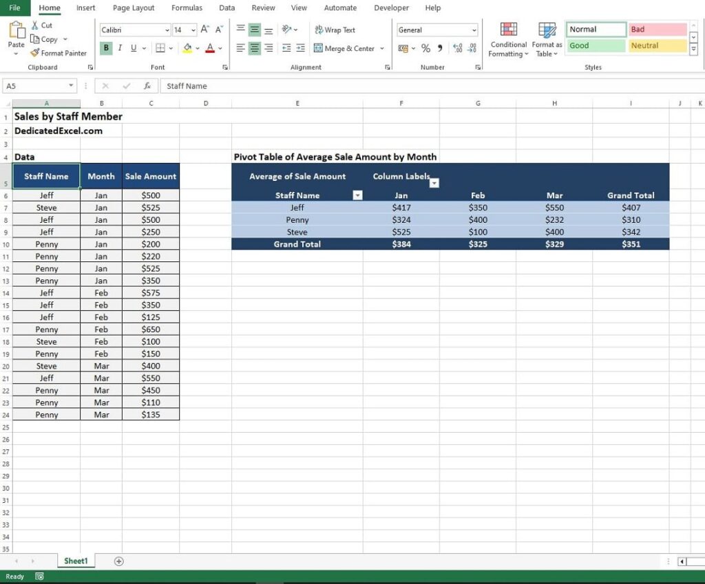
In this example, we have a basic Q1 Sales Report featuring ‘Staff Name‘, ‘Month‘, and ‘Sale Amount‘. Using this data, we have created a Pivot table that neatly displays the ‘Average Sale by Month‘ for each staff member.
Here’s where the magic happens: Our goal is to ensure that as new data, like April’s Sales, gets added to the Sales Report, we won’t have to tweak our Pivot table’s data range. Instead, we want to simply hit ‘Refresh‘, and voila! The Pivot table will automatically recognize and incorporate the new data in our Sales Report.
Step 1 – Convert the Data to an Excel Table
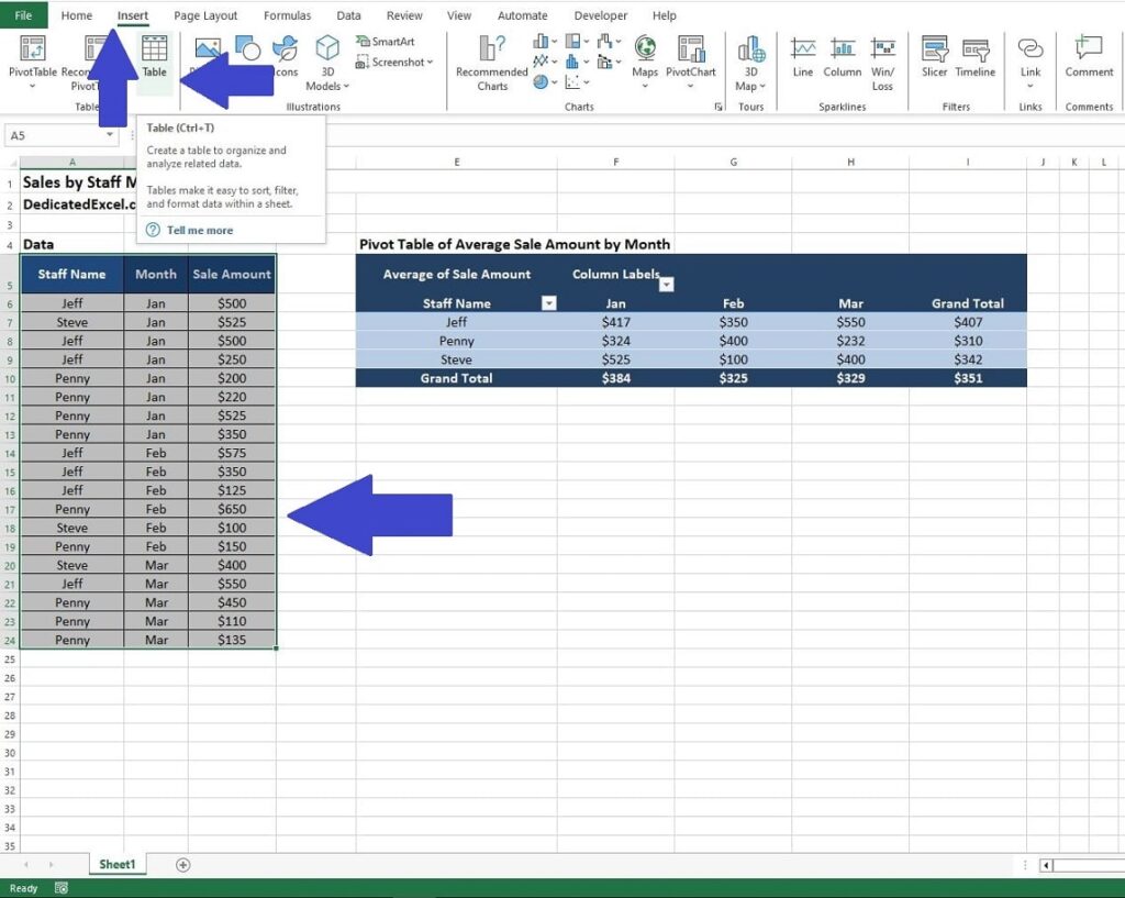
The first step in the process to make our Pivot table update automatically is to convert our Sales data, found in cells A5:C24 of the example, into an Excel Table. This is a crucial step in the process as by nature Tables in Excel automatically expand to include new data.
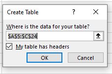
First, highlight the data range (A5:C24) then on the Excel Ribbon go to the ‘Insert‘ tab and click on ‘Table’. That will bring up the ‘Create Table‘ settings which is where we can decide to change the data range, or uncheck whether headers are included within that range.
For this example no changes are required as we already highlighted the correct data range, click ‘OK‘ and Excel will convert the range into a Table.
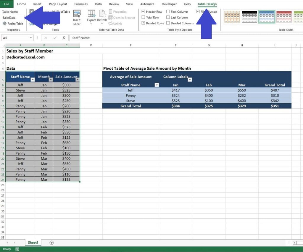
If you have completed the step correctly you’ll notice some basic formatting changes to the data range, and the headers now have drop-down arrows for sorting and filtering. Click anywhere in the Table and, making sure you are in the ‘Table Design‘ tab on the Excel ribbon, make a note of the ‘Table Name‘ on the far left of the screen.
By default Excel will give names like ‘Table1’, ‘Table2’, ‘Table3’ etc, when you create a new Table. It’s good practice to use a meaningful name for better readability and easier reference. For this example we can replace ‘Table1‘ with ‘SalesData‘. Remember this name as we’ll need it later.
There are some constraints and best practices to be aware of when choosing a Table name in Excel, especially when setting up your data for a pivot table update automatically.
- Uniqueness: The table name must be unique within the workbook. You cannot have two tables with the same name.
- No Spaces: Table names cannot contain spaces. Use underscores (_) or CamelCase (e.g., SalesData) for multi-word names.
- Avoid Special Characters: It’s best to avoid special characters like #, &, or $. Stick to letters, numbers, and underscores.
- No Excel Reserved Words: Avoid using names that Excel uses for its own features, like ‘History’, ‘Table’, etc.
- Descriptive Names: Choose a name that describes the data in the table. For instance, for a table containing Q1 sales data, you might name it ‘Q1SalesData’.
- Length Limit: The name should not be excessively long. Keep it concise yet descriptive.
Step 2 – Create Pivot Table
For our example we have already created a basic Pivot table that we want to make dynamic. If you haven’t already created a Pivot table to display your data you should do so at this stage.
We won’t cover all the step-by-step guide to that process in this post, but you can refer to the guide on Excel Pivot Tables and How to Create One if you need a detailed assistance with this.
Step 3 – Making the Pivot Table Dynamic
With the data now neatly organized into an Excel Table and our Pivot Table set up, we’re just one step away from syncing the two. By linking the Excel Table with the Pivot Table, we create a dynamic setup in Excel.
This step ensures that our Pivot Table automatically adjusts its data range whenever new information is added to the Sales report, eliminating the need for manual updates and maintaining a consistently up-to-date analysis.
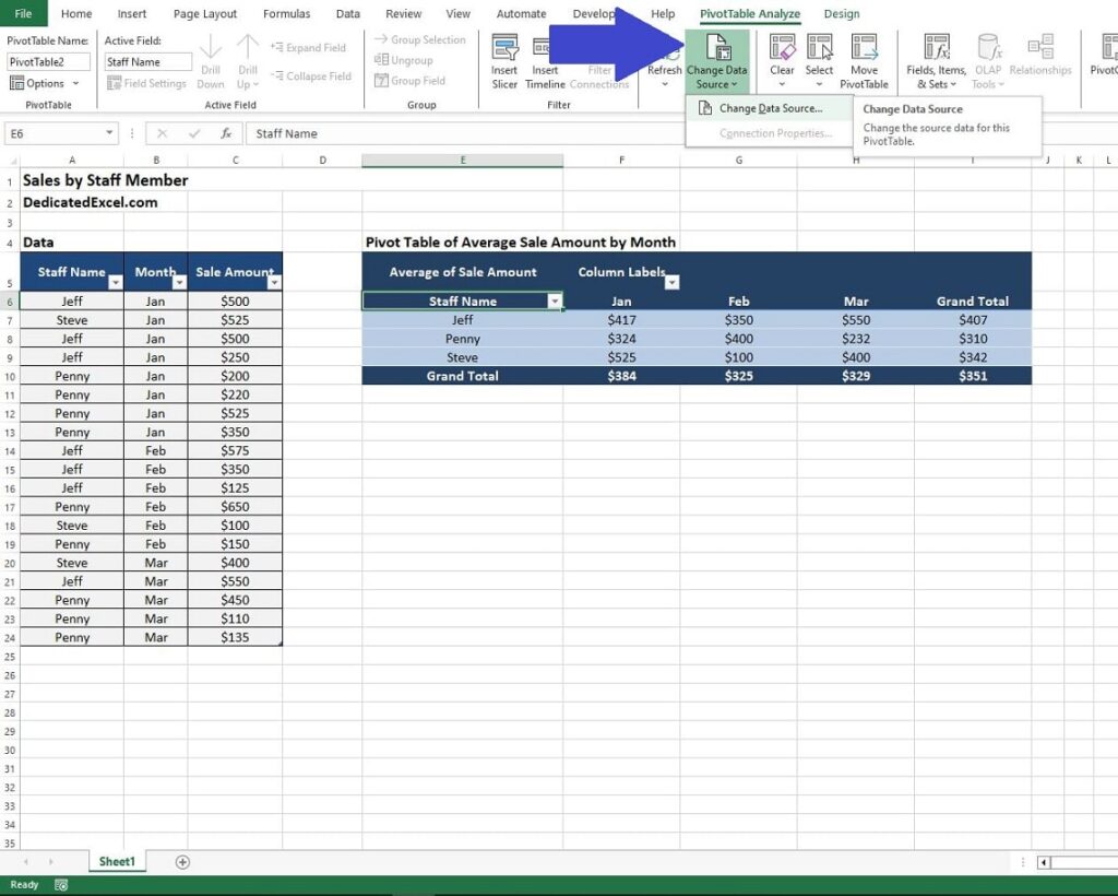
First, click on any cell in the existing Pivot Table and then navigate to the ‘PivotTable Analyze‘ tab on the Excel ribbon. From there select the option to ‘Change Data Source‘.
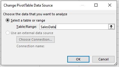
In the Table/Range criteria we need to replace the existing data range for A5:C24 with our Excel Table, created in Step 1. If you remember we called this ‘SaleData‘ so in the criteria box type ‘SalesData‘ and click ‘OK‘.
Step 4 – Test the Dynamic Pivot Table
Finally, we test the new settings to ensure everything has been set-up correctly.
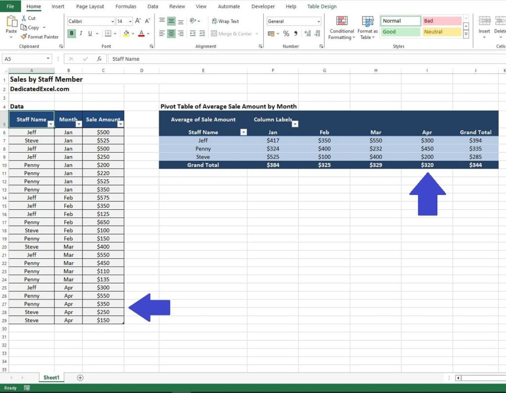
If we add in some April Sales figures to rows 25 to 30, you should notice your Table formatting expands with the new data, confirming to you that it is being included.
With some new data added we can test the dynamic Pivot table by right-clicking on the Pivot table, then select ‘Refresh‘. If everything has worked you’ll see the new Average Sales Amounts for April added to the Pivot table automatically.
Factors to Consider with Dynamic Pivot Tables
When you set out to make Excel Pivot Table update automatically, it’s not just about the technical steps. There are several key factors to consider to ensure that your dynamic Pivot table is both efficient and effective:
Data Quality and Consistency
- Clean Data: Ensure your data is clean and well-organized before converting it into a Table. Inconsistent or erroneous data can lead to misleading Pivot table results.
- Consistent Formatting: Consistency in data entry (like date formats, categorizations) is crucial. Inconsistencies can cause issues in data representation and analysis in the Pivot table.
Table Structure
- Header Clarity: Each column in your Excel Table should have a clear, unique header. This aids in accurately setting up your Pivot table fields.
- Avoiding Blank Rows/Columns: Blank rows or columns within your data can disrupt the Table and Pivot table’s ability to correctly interpret the data range.
Data Range Expansion
- Anticipate Growth: When converting a data range into a Table, remember that the Table will expand as new data is added. Ensure there’s enough space in your worksheet to accommodate this growth without interfering with other data or tables.
PIVOT Table Refreshing
- Regular Refreshes: After making your Pivot table dynamic, it’s important to refresh it regularly to ensure it includes the latest data.
- Automatic vs Manual Refresh: Consider using Excel’s automatic refresh options if your data source is linked to external data. For local data, manual refreshing after adding new data might be necessary.
Performance Considerations
- Large Data Sets: Be mindful of the size of your data. Extremely large datasets can slow down the performance of your Pivot table.
- Calculated Fields and Items: Use calculated fields and items judiciously, as they can also impact performance.
Data Security and Control
- Access Control: If your Excel file is shared, consider who has access to modify the data. Changes in the source data can affect your Pivot table outputs.
- Data Validation: Regularly validate your data to maintain the integrity of your reports.
By keeping these factors in mind, you not only make your Excel Pivot table update automatically, but also a reliable and powerful tool for data analysis.
Summary
In conclusion, mastering how to make Excel Pivot table update automatically is more than just a time-saving skill; it’s about enhancing your efficiency and accuracy in handling data. This guide has walked you through the essential steps of converting your data into a dynamic Table and linking it seamlessly with a Pivot table. By doing so, you’ve set the stage for automatic updates, ensuring that your data analysis remains current and relevant without the need for constant manual adjustments.
Remember, the power of a dynamic Pivot table lies in its ability to adapt to new data effortlessly. This capability not only streamlines your workflow but also minimizes the chances of errors that can occur with manual updates. Whether you’re creating reports for business, academic, or personal use, the dynamic Pivot table you’ve learned to create today will serve as a robust tool in your Excel toolkit.
Keep Excelling,

As you’ve learned to make your pivot table update automatically, embracing the efficiency of dynamic Excel Pivot tables, why not elevate your skills even further? Our next guide, ‘How to Count Unique Records in a Pivot Table,’ awaits your exploration. This tutorial unlocks another powerful aspect of Excel, allowing you to extract even deeper insights from your automatically updating data. Ideal for managing extensive datasets or simply enhancing your data organization skills, mastering the counting of unique records in your dynamic Pivot table is an invaluable addition to your Excel toolkit.