
Master the art of crafting a dynamic chart title in Excel with our step-by-step guide. Perfect for evolving data, this technique automates your chart titles, ensuring they’re always current without manual effort. Save time and enhance your Excel skills today.
Introduction
Excel’s capability to transform data into visually compelling charts is a game-changer for data analysis and presentation. As an Excel developer, whether you’re building detailed reports, interactive dashboards, or ad-hoc MI reports, the importance of the chart title cannot be overstated. It’s the first thing users notice and sets the context for the data being presented.
However, it’s not uncommon to see charts with missing or outdated titles. This oversight can lead to confusion or misinterpretation of the data, diminishing the value of your hard work.
Dynamic chart titles
The key to maintaining accurate and relevant Excel charts lies in employing dynamic chart titles. A dynamic chart title dynamically links to a specific cell within your Excel sheet. This means the chart title automatically reflects the content of this reference cell, such as “Sales Overview“.
While it might initially seem trivial, this feature becomes incredibly powerful when utilized effectively. Imagine a chart title that automatically updates to show the latest date range or data subset, significantly reducing manual updates and ensuring your charts always tell the current story.
Example
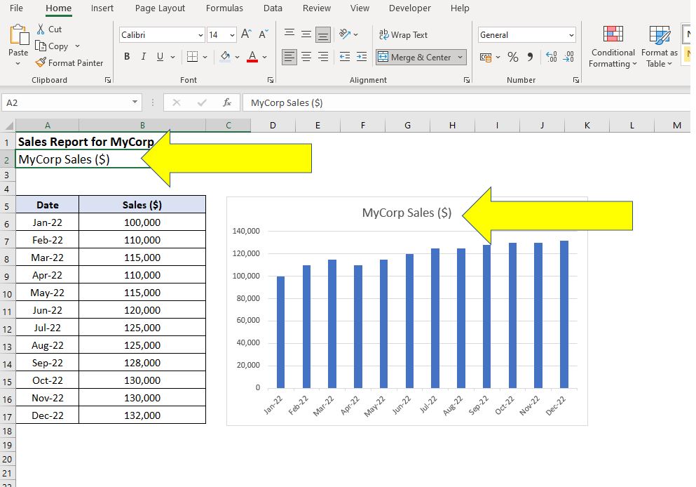
To illustrate dynamic chart titles in Excel consider the following sales report where a standard column chart has been included to visualize the sales figures:
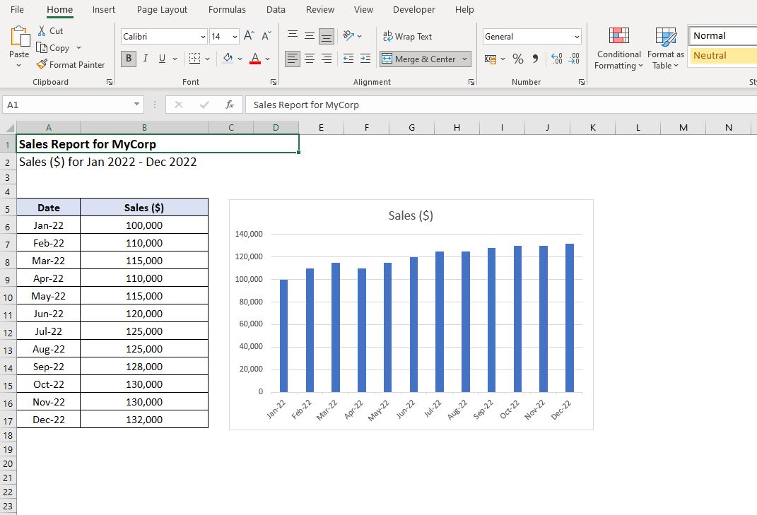
Excel automatically includes the chart title Sales ($) as this is the value illustrated on the chart but that is not very descriptive, as an Excel developer its possible to do better and link the chart title to a cell.
In this example the cell A2 contains a more descriptive version of what is shown. Sales ($) for Jan 2022 – Dec 2022 so cell A2 becomes the reference cell.
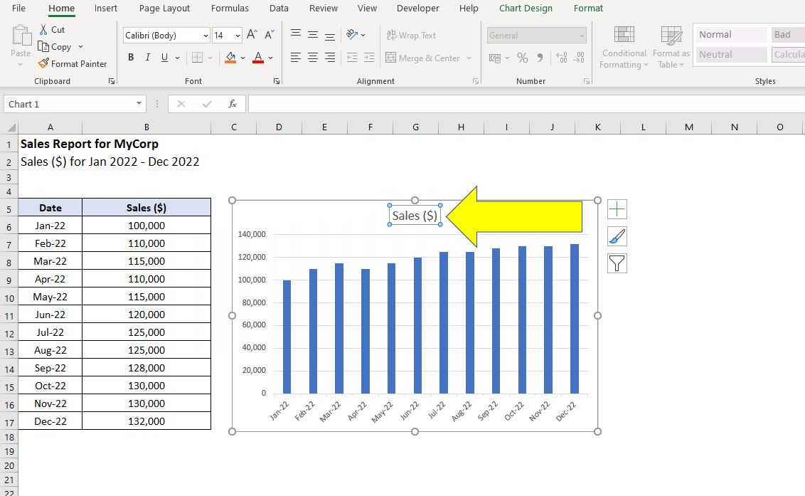
To link the chart title to this cell first click on the chart title so it becomes highlighted:
The following step involves clicking on the formula bar and specifying the reference cell’s location, which, in our example, is cell A2. It’s crucial to include the worksheet name in this formula. So, if your worksheet is named ‘Sheet1‘, the formula you need to enter would be:
- = Sheet1!$A$2
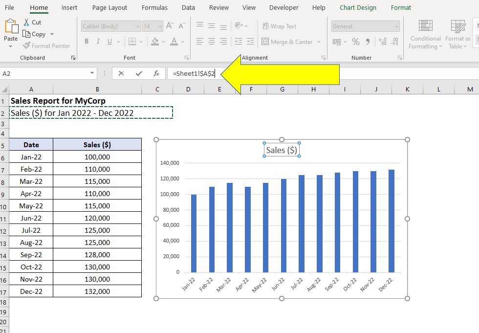
Next, press enter and the chart title will update to the content from cell A2:
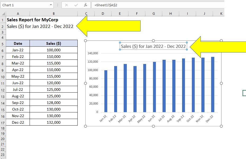
The Excel chart title is now dynamic. Should you modify cell A2, for instance, changing it to ‘MyCorp Sales ($)‘, the chart title will automatically update to reflect this change:
Summary
In this post, we’ve explored the steps to create dynamic chart titles in Excel, a vital skill for effective data visualization. By linking chart titles to cell references, your charts remain up-to-date, reflecting changes in data instantly. This technique not only saves time but also ensures accuracy, making your Excel charts more intuitive and user-friendly.
Remember, dynamic titles are just the beginning; there’s a world of Excel functionalities waiting to be discovered!
Keep Excelling,

Just mastered dynamic chart titles in Excel? Elevate your Excel efficiency further with ‘5 Time-Saving Techniques for Excel‘. Dive in to discover more expert tips and tricks that streamline your workflow.