
Have you ever felt overwhelmed while trying to find specific data in a large Excel spreadsheet? Imagine you’re staring at a sea of numbers and columns, wishing there was a magic wand to instantly pinpoint the information you need. Well, there’s no magic wand, but there’s something equally powerful in Excel, and it’s called the HLOOKUP function. In this beginner-friendly guide, I’ll walk you through how to use HLOOKUP in Excel, a tool that promises to instantly transform your data searching skills and make you an Excel pro today!
Table of Contents
- What is HLOOKUP?
- Why use HLOOKUP?
- HLOOKUP or VLOOKUP in Excel?
- The HLOOKUP Function in Excel
- Example – Create an Inventory Checker
- Common Mistakes
- Tips for using HLOOKUP in Excel
- Summary
What is HLOOKUP in Excel?
HLOOKUP stands for Horizontal Lookup. It’s a function in Excel that enables you to search for a value in the top row of a table or range and return a value in the same column from a row you specify.
In simpler terms, it’s like playing a matching game: HLOOKUP finds the row that matches your search and retrieves the data you need from that row.
Why Use HLOOKUP in Excel?
Imagine you have a spreadsheet filled with sales data for different products across several months. If you need to find out the sales figures for a specific product in a specific month, sifting through each column can be tiresome. HLOOKUP does this job for you in seconds. It’s not just a time-saver; it ensures accuracy in data retrieval, which is crucial in any professional scenario.
HLOOKUP or VLOOKUP?
When it comes to Excel, choosing between HLOOKUP and VLOOKUP depends on the orientation of your data and the specific requirements of your task. Both functions serve similar purposes – searching for and retrieving data based on a specified criterion – but they operate in different directions.
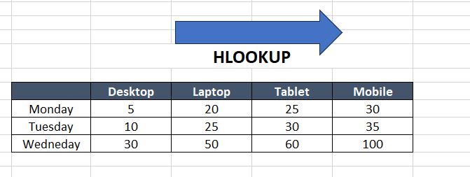
HLOOKUP (Horizontal Lookup)
HLOOKUP is used when your data is organized horizontally, with the criteria or keys located in the top row. HLOOKUP searches for a specified value in the first row of a table array and retrieves a corresponding value from a specified row.
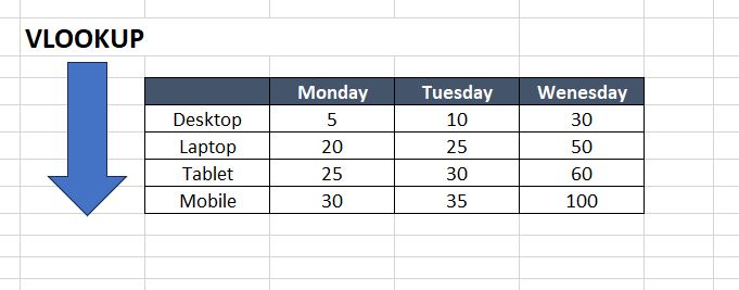
VLOOKUP (Vertical Lookup)
VLOOKUP, on the other hand, is designed for data that is organized vertically, with the criteria or keys located in the leftmost column. VLOOKUP searches for a specified value in the first column of a table array and retrieves a corresponding value from a specified column.
The HLOOKUP Function in Excel
The basic syntax of HLOOKUP is as follows:
- =HLOOKUP(lookup_value, table_array, row_index_num, [range_lookup])
- lookup_value: The value you want to search for.
- table_array: The range of cells where the search will be performed.
- row_index_num: The row number in the table from which to retrieve the value.
- [range_lookup]: Optional. Use FALSE to find an exact match and TRUE for an approximate match. If you omit this, TRUE is the default.
Example – Create an Inventory Checker using HLOOKUP
HLOOKUP Example File Download
To master the HLOOKUP function in Excel, let’s dive into an easy-to-follow example. For a hands-on experience, feel free to download the example file and follow along by clicking the button below:
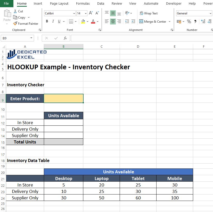
Download HLOOKUP Example FileLet’s simplify our example by creating an Inventory Checker. This tool will help us quickly find out the number of units for any product. Here’s how it works:
- Enter a product name in cell B9.
- Instantly see the available units:
- ‘In-Store‘ in cell B12
- ‘Delivery Only‘ in cell B13
- ‘Supplier Only‘ in cell B14
- ‘Total Units‘ in cell B15
- We’ll use Excel’s HLOOKUP function to fetch these unit totals from our ‘Inventory Data Table‘ located in cells A21 to E24.
Enter the Formulas using the HLOOKUP Function
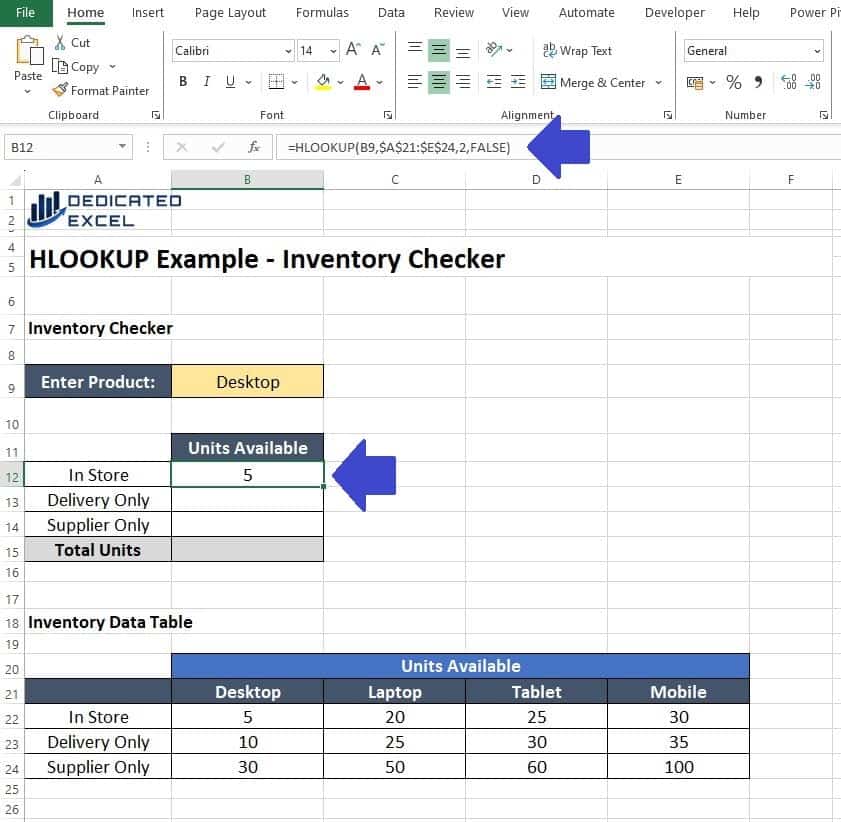
To begin let’s populate cell B9 with a ‘Product‘, this will help to ensure our formula’s are working as we build them. In cell B9 enter the text “Desktop“.
Next, let’s set up the initial formula to display the in-store inventory levels for the selected product. Enter this formula in cell B12, and you should see the number ‘5‘ appear as the result.
- =HLOOKUP(B9,$A$21:$E$24,2,FALSE)
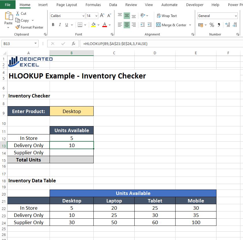
The next formula to complete is for the ‘Delivery Only’ inventory levels. In cell B13 enter the following formula, using the HLOOKUP function in Excel. The result should appear as ‘10‘.
- =HLOOKUP(B9,$A$21:$E$24,3,FALSE)
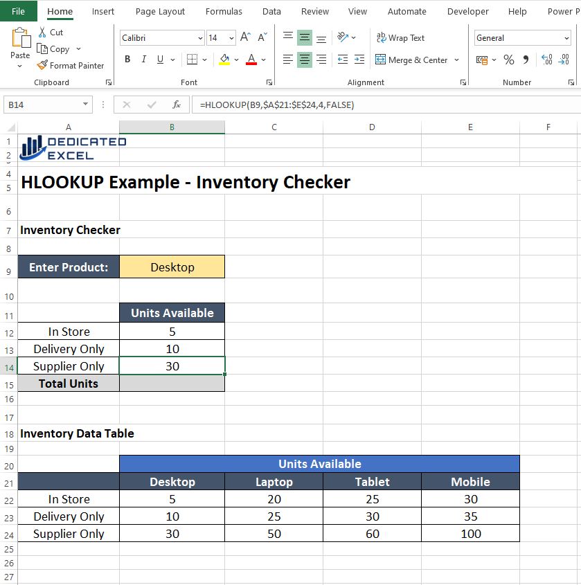
The third formula in our inventory checker is in cell B14, this will display the inventory available via the Supplier. In cell B14 enter the following formula and the result should be ‘30‘.
- =HLOOKUP(B9,$A$21:$E$24,4,FALSE)
Finally to finish off we can use the SUM function in Excel to determine the ‘Total Units‘. To do so in cell B15 enter the following formula:
- =SUM(B12:B14)

Testing the Results
We can test our Inventory Checker in action by changing the ‘Product‘ in cell B9 to one of the others we sell, ‘Laptop‘, ‘Tablet‘ or ‘Mobile‘.
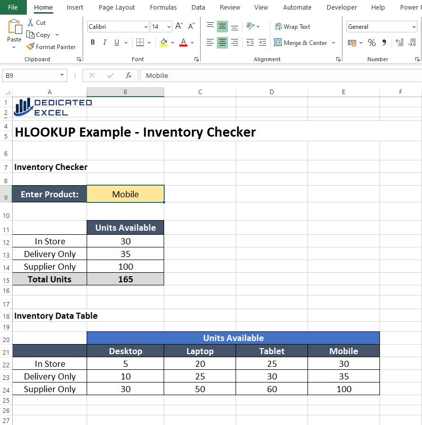
Let’s test by entering the text “Mobile” in cell B9.
The Inventory Checker should show:
- 30 units available in-store
- 35 units delivery only
- 100 units available from the supplier
- a total of 165 available units.
Awesome job!
It looks like you have mastered how to use the HLOOKUP function in Excel.

Common Mistakes with HLOOKUP
When working with HLOOKUP in Excel, it’s essential to navigate past the common errors that many users encounter. These mistakes can easily disrupt your data analysis process.
Let’s break down some of the most frequent missteps and learn how to avoid them:
Understanding Match Types
The range_lookup argument is critical in HLOOKUP. For precise results, set it to FALSE when you need an exact match. For instance, if you’re looking for “Product B” in a horizontal table, your formula should look like =HLOOKUP(“Product B”, A1:E5, 2, FALSE). Remember, using TRUE for approximate matches might lead to unexpected outcomes.
Correct Data Orientation
HLOOKUP is tailor-made for horizontal data layouts. A common blunder is attempting to use it on vertically arranged data. This mismatch will lead to errors. Make sure your data is set up horizontally. If your data is vertical, you might want to explore How to Use a VLOOKUP in Excel instead.
Accurate Row Indexing
A frequent error with HLOOKUP is selecting the incorrect row index in your formula. This mistake can lead to misleading results. For example, if you’re trying to find sales data for “Product C”, an incorrect row reference will fetch the wrong information.
Comprehensive Table Array
Your table array should encompass all the data you wish to search through. If your array is incomplete, you might miss vital information, leading to inaccurate findings. Ensure your table array is fully defined to include every relevant piece of data.
By paying close attention to these areas, you can use HLOOKUP more effectively, ensuring that your Excel work is both accurate and efficient. Remember, mastering these details is a key step in becoming proficient with Excel’s powerful data retrieval functions.
Tips for Using HLOOKUP in Excel
While HLOOKUP in Excel is a powerful tool, employing a few strategic tips can significantly elevate your data retrieval process. Here’s how:
- Utilize Named Ranges for Enhanced Clarity: To make your HLOOKUP formulas more readable and manageable, use named ranges. For instance, create a named range like “SalesData” for your table array. This approach simplifies your formula to something like =HLOOKUP(“Product B”, SalesData, 2, FALSE), making it more intuitive and easier to understand.
- Incorporate Error Handling for a User-Friendly Experience: Use error-handling functions like IFERROR in your HLOOKUP formulas. This step is crucial for providing clear messages or alternative instructions when HLOOKUP fails to find a match. It greatly improves the user experience by preventing confusing error messages and maintaining the functionality of your spreadsheet.
- Ensure Data Validation for Increased Reliability: Prior to applying HLOOKUP, it’s important to validate and tidy up your data. Removing duplicates and inconsistencies is key to obtaining reliable and accurate results. Data that is well-organized and validated ensures that your lookups are both precise and dependable.
By integrating these tips into your Excel practice, you can effectively leverage HLOOKUP for detailed and efficient data analysis. These strategies not only help in avoiding common mistakes but also enhance the overall functionality and user experience of your spreadsheets. Keep these insights in mind to harness the full potential of HLOOKUP in your Excel endeavours.
Summary
As we conclude our exploration of HLOOKUP in Excel, let’s recap the essential takeaways from this post:
- Understanding HLOOKUP: We delved into what HLOOKUP is and how it’s a valuable tool for horizontal data searching in Excel.
- Practical Application: Through our step-by-step guide, we demonstrated how to use HLOOKUP effectively, using our Inventory Checker example for practical learning.
- Common Mistakes: We addressed typical errors like match type confusion, data layout mismatch, row reference errors, and incomplete table arrays, offering solutions to avoid them.
- Helpful Tips: We explored tips such as using named ranges for clarity, implementing error handling for better user experience, and ensuring data validation for reliable results.
By now, you should feel more confident in your ability to use HLOOKUP in Excel, equipped with the knowledge to avoid common mistakes and apply best practices. Whether you’re a beginner or an experienced Excel user, mastering HLOOKUP can significantly enhance your data analysis and retrieval skills. Keep practicing, and soon you’ll be leveraging HLOOKUP like a pro!
Keep Excelling,

.
Just mastered HLOOKUP in Excel and feeling like an Excel wizard? Keep the momentum going and take a step further towards a more comfortable Excel experience. Don’t miss our next post, ‘Enable Dark Mode in Excel for Eye-Friendly Work‘, where you’ll learn how to switch to a soothing, eye-friendly interface. Say goodbye to eye strain and hello to a sleek, modern Excel look!